Cloth Simulation with Root Finding and Optimization
0 前言
声明:此篇博客仅用于个人学习记录之用,并非是分享代码。Hornor the Code
我只能说,衣料模拟的技术深度比3D刚体模拟的技术深太多了。这次的实验参考了许多资料,包括
- 《University of Tennessee MES301 Fall, 2023》
- 《Root finding and optimization: Scientific Computing for Physicists 2017》
- 《Physics-based animation lecture 5: OH NO! It's More Finite Elements》 这个老师讲课用一个小猫,特逗
- 当然主要还是 Games103王华民老师的《Intro to Physics-Based Animation!》
里面用到的一些技术,在有限元里也有应用。
另外还有不基于物理的衣料模拟 《Position Based Dynamics》, 这个是05年左右开始出现的技术。详细的内容可以看PBA 2014: Position Based Dynamics by Ladislav Kavan,因为不基于物理,这里不再涉及。
1 Implicit Method
\]
进行一些简单的变换。
\]
这里,我们只是认为力是位置的函数,所以可以写成。
\]
这就需要解一个非线性方程,其中力并非是线性的。
In mathematics and science, a nonlinear system (or a non-linear system) is a system in which the change of the output is not proportional to the change of the input.
In mathematics, a linear map (or linear function) \(f(x)\) is one which satisfies both of the following properties:\[\bullet\text{ Homogeneity: }f(\alpha x)=\alpha f(x).
\]\[\bullet\text{Additivity or superposition principle:}f(x+y)=f(x)+f(y);
\]
\]
\]
上面的式子其实是求出了隐式积分的原函数,上式求导就是隐式积分本身。
\]
所以一个求解非线性方程,或者是求解非线性方程根的模式就可以变成优化问题,而且是非线性优化。
1.1 Root-finding
The solution of nonlinear algebraic equations is frequently called root-finding, since our goal is to find the value of \(x\) such that $$f(x) = 0.$$
1.2 Optimization
Optimization means finding a maximum or minimum.
In mathematical terms, optimization means finding where the derivative is zero.
\]
University of Tennessee MES301
Root finding and optimization: Scientific Computing for Physicists 2017
1.3 Insight
我们看到,这两个东西很像,基本就是解方程。所以有时候我们可以将其进行转化。
就是导数和积分的关系。
Physics-based animation lecture 5: OH NO! It's More Finite Elements
2 Newton-Raphson Method
Given a current \(\mathbf{x}^{(k)}\), we approximate our goal by:
\]
We then solve:
\]
\]
Specifically to simulation, we have:
F(\mathbf{x})=\frac1{2\Delta t^2}\|\mathbf{x}-\mathbf{x}^{[0]}-\Delta t\mathbf{v}^{[0]}\|_{\mathbf{M}}^2+E(\mathbf{x}) \\
\nabla F\left(\mathbf{x}^{(k)}\right)=\frac1{\Delta t^2}\mathbf{M}\left(\mathbf{x}^{(k)}-\mathbf{x}^{[0]}-\Delta t\mathbf{v}^{[0]}\right)-\mathbf{f}\left(\mathbf{x}^{(k)}\right)\\
\frac{\partial F^2\left(\mathbf{x}^{(k)}\right)}{\partial\mathbf{x}^2}=\frac1{\Delta t^2}\mathbf{M}+\mathbf{H}(\mathbf{x}^{(k)})
\end{gathered}
\]
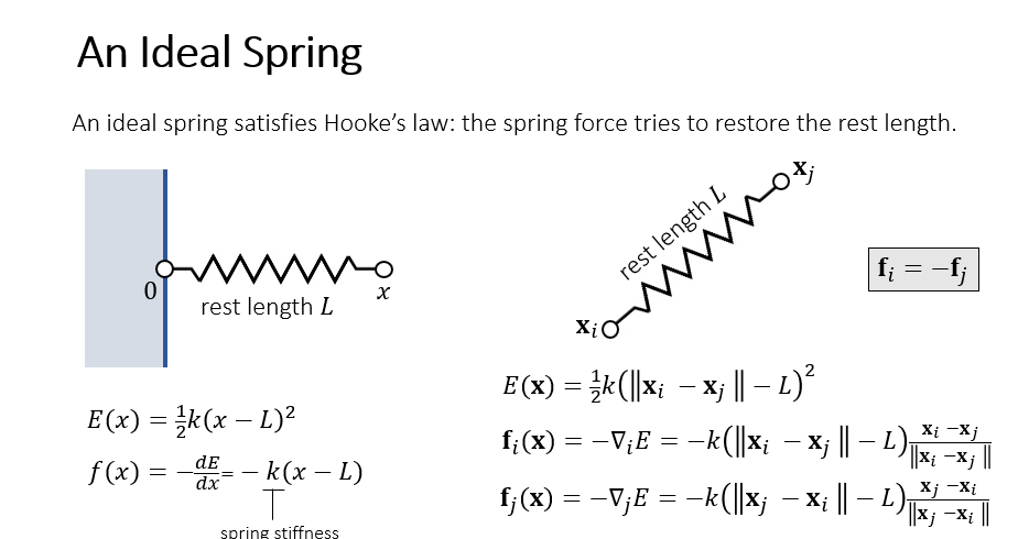
3 Mass-Spring System
\]
\]
3.1 Matrix calculus
\]
\]
\]
\]
3.2 A Spring with Two Ends
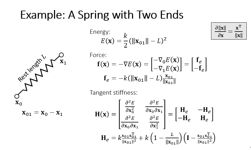
图片来源:Games103
4 Explaination of Init Code with 3D Image
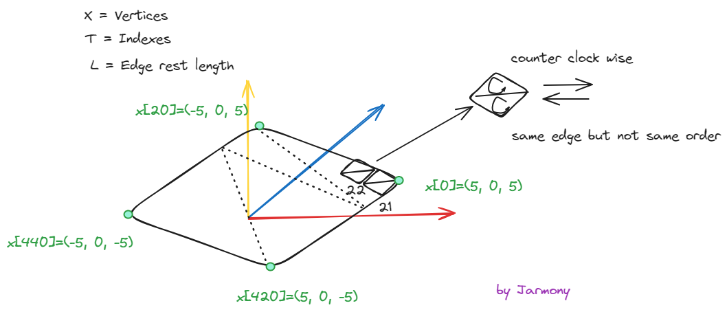
4.1 Initialize
void Start(){Mesh mesh = GetComponent<MeshFilter> ().mesh;//Resize the mesh.int n=21;Vector3[] X = new Vector3[n*n];Vector2[] UV = new Vector2[n*n];int[] triangles = new int[(n-1)*(n-1)*6];for(int j=0; j<n; j++)for(int i=0; i<n; i++){X[j*n+i] =new Vector3(5-10.0f*i/(n-1), 0, 5-10.0f*j/(n-1));UV[j*n+i]=new Vector3(i/(n-1.0f), j/(n-1.0f));}int t=0;for(int j=0; j<n-1; j++)for(int i=0; i<n-1; i++){triangles[t*6+0]=j*n+i;triangles[t*6+1]=j*n+i+1;triangles[t*6+2]=(j+1)*n+i+1;triangles[t*6+3]=j*n+i;triangles[t*6+4]=(j+1)*n+i+1;triangles[t*6+5]=(j+1)*n+i;t++;}mesh.vertices=X;mesh.triangles=triangles;mesh.uv = UV;mesh.RecalculateNormals ();Debug.Log("triangles.Length " + triangles.Length);//Construct the original Eint[] _E = new int[triangles.Length*2];Debug.Log("_E.Length " + _E.Length);for (int i=0; i<triangles.Length; i+=3){_E[i*2+0]=triangles[i+0];_E[i*2+1]=triangles[i+1];_E[i*2+2]=triangles[i+1];_E[i*2+3]=triangles[i+2];_E[i*2+4]=triangles[i+2];_E[i*2+5]=triangles[i+0];}//Reorder the original edge listfor (int i=0; i<_E.Length; i+=2)if(_E[i] > _E[i + 1])Swap(ref _E[i], ref _E[i+1]);//Sort the original edge list using quicksort// One edge have two end point, this quicksort method sort all of them at the same time// the order is from small to big with the pattern of// [start end] [start end] [start end]//Debug.Log("_E.Length/2-1 " + (_E.Length / 2 - 1) );Quick_Sort(ref _E, 0, _E.Length/2-1);// short-circuit evaluation: or(if first condition is true then skip other) and(if first condition is false then skip other)int e_number = 0;for (int i=0; i<_E.Length; i+=2)if (i == 0 || _E [i + 0] != _E [i - 2] || _E [i + 1] != _E [i - 1])e_number++;E = new int[e_number * 2];for (int i=0, e=0; i<_E.Length; i+=2)if (i == 0 || _E [i + 0] != _E [i - 2] || _E [i + 1] != _E [i - 1]){E[e*2+0]=_E [i + 0];E[e*2+1]=_E [i + 1];e++;}// [0-9] 10/2=5 <5=4 4*2+1=9// [0-10] 11/2=5 <5=4 4*2+1=9// asert(E.length % 2 == 0) this should always be true, becuase we use one dim array to store the Edges. One edge takes two places in this array.L = new float[E.Length/2];for (int e=0; e<E.Length/2; e++){int v0 = E[e*2+0];int v1 = E[e*2+1];L[e]=(X[v0]-X[v1]).magnitude;}V = new Vector3[X.Length];for (int i=0; i<V.Length; i++)V[i] = new Vector3 (0, 0, 0);}
4.2 Index
int t=0;// Because of 21 points have 20 gaps, this index will iterate 400 squares and split them two triangels// per square.for(int j=0; j<n-1; j++)for(int i=0; i<n-1; i++){triangles[t*6+0]=j*n+i;triangles[t*6+1]=j*n+i+1;triangles[t*6+2]=(j+1)*n+i+1;triangles[t*6+3]=j*n+i;triangles[t*6+4]=(j+1)*n+i+1;triangles[t*6+5]=(j+1)*n+i;t++;}
这里的 triangles 其实就是 三角形顶点的Index(下标)。
State: j=0, i=0, t=0.t[0] = 0t[1] = 1t[2] = 22t[3] = 0t[4] = 22t[5] = 21/*********/State: j=0, i=1, t=1.t[6] = 1t[7] = 2t[8] = 23t[9] = 1t[10] = 23t[11] = 22
4.3 Edge
//Construct the original Eint[] _E = new int[triangles.Length*2];Debug.Log("_E.Length " + _E.Length);for (int i=0; i<triangles.Length; i+=3){_E[i*2+0]=triangles[i+0];_E[i*2+1]=triangles[i+1];_E[i*2+2]=triangles[i+1];_E[i*2+3]=triangles[i+2];_E[i*2+4]=triangles[i+2];_E[i*2+5]=triangles[i+0];}//Reorder the original edge listfor (int i=0; i<_E.Length; i+=2)if(_E[i] > _E[i + 1])Swap(ref _E[i], ref _E[i+1]);
因为这里使用一维数组进行边的存储,那么从一条边到另一条边的步长是2。
State: i=0._E[0] = t[0]:0_E[1] = t[1]:1_E[2] = t[1]:1_E[3] = t[2]:22_E[4] = t[2]:22_E[5] = t[0]:0/*********/State: i=3._E[6]= t[3]:0_E[7] = t[4]:22_E[8] = t[4]:22_E[9] = t[5]:21_E[10] = t[5]:21_E[11] = t[3]:0
4.4 Sort Edge
//Reorder the original edge listfor (int i=0; i<_E.Length; i+=2)if(_E[i] > _E[i + 1])Swap(ref _E[i], ref _E[i+1]);
初始的时候,一条边有两种表达方式。我们将其都按从小的顶点到大的顶点进行重新排序,一条边就只有一种表达方式。
Quick_Sort(ref _E, 0, _E.Length/2-1);void Quick_Sort(ref int[] a, int l, int r){int j;if(l<r){j=Quick_Sort_Partition(ref a, l, r);Quick_Sort (ref a, l, j-1);Quick_Sort (ref a, j+1, r);}}int Quick_Sort_Partition(ref int[] a, int l, int r){int pivot_0, pivot_1, i, j;pivot_0 = a [l * 2 + 0];pivot_1 = a [l * 2 + 1];i = l;j = r + 1;//Debug.Log("i: " + i + " j:" + j);while (true){do ++i; while( i<=r && (a[i*2]<pivot_0 || a[i*2]==pivot_0 && a[i*2+1]<=pivot_1));do --j; while( a[j*2]>pivot_0 || a[j*2]==pivot_0 && a[j*2+1]> pivot_1);if(i>=j) break;Swap(ref a[i*2], ref a[j*2]);Swap(ref a[i*2+1], ref a[j*2+1]);}Swap (ref a [l * 2 + 0], ref a [j * 2 + 0]);Swap (ref a [l * 2 + 1], ref a [j * 2 + 1]);return j;}void Swap(ref int a, ref int b){int temp = a;a = b;b = temp;}
这里的quick sort是以两个数为一次比较的依据,好像是这两个数打包(其实就是一条边)进行比较,平常就是一次比较只关心一个数。
5 Update
// Update is called once per framevoid Update (){Mesh mesh = GetComponent<MeshFilter> ().mesh;Vector3[] X = mesh.vertices;Vector3[] last_X = new Vector3[X.Length];Vector3[] X_hat = new Vector3[X.Length];Vector3[] G = new Vector3[X.Length];//Initial Setup.for (int i = 0; i < X.Length; i++){if (i == 0 || i == 20) continue;V[i] = V[i] * damping;X_hat[i] = X[i] + V[i] * t;last_X[i] = X[i];// Guess X[i] init stateX[i] = X_hat[i];}float invSquareDt = 1 / (t * t);// Hessian Matrix is complicated to construct// So we use some fake inverse, due to the mass is same for all vertices, we put this out of the loop.float fakeInv = 1 / (invSquareDt * mass + 4.0f * spring_k);for (int k=0; k<32; k++){Get_Gradient(X, X_hat, t, G);//Update X by gradient.for (int i = 0; i < X.Length; i++){if (i == 0 || i == 20) continue;X[i] = X[i] - fakeInv * G[i];}}float invTime = 1.0f / t;for (int i = 0; i < X.Length; i++){if (i == 0 || i == 20) continue;V[i] = invTime * (X[i] - last_X[i]);}//Finishing.mesh.vertices = X;Collision_Handling ();mesh.RecalculateNormals ();}
因为要进行优化,位置迭代,来找到最小值。所以需要一个迭代的初始位置,设置为X_init = X[i] + V[i] * t。也可以不设置,不进行变化。
6 Get_Gradient
void Get_Gradient(Vector3[] X, Vector3[] X_hat, float t, Vector3[] G){//Momentum and Gravity.float invSquareDt = 1 / (t * t);for (int i = 0; i < X.Length; i++){G[i] = invSquareDt * mass * (X[i] - X_hat[i]) - mass * gravity;}//Spring Force.Vector3 spForceDir = Vector3.zero;Vector3 spForce = Vector3.zero;for (int e = 0; e < E.Length / 2; e++){int vi = E[e * 2 + 0];int vj = E[e * 2 + 1];spForceDir = X[vi] - X[vj];spForce = spring_k * (1.0f - L[e] / spForceDir.magnitude) * spForceDir;G[vi] = G[vi] + spForce;G[vj] = G[vj] - spForce;}}
6.1 first derivative
\]
由于上式的特性,我们需要两次遍历来得到梯度一阶导的数值。
- 逐顶点
\]
- 逐边计算弹簧弹力
\]
当然无论是逐顶点还是逐边,导数都是位置的函数。
最后给每一个顶点的梯度加上重力,当然根据 g 需要加负号。
6.2 second derivative
In reality, there are two roadblocks:
1)The Hessian matrix is complicated to construct;
2) the linear solver is difficult to implement on Unity.
Instead, we choose a much simpler method by considering the Hessian as a diagonal matrix. This
yields a simple update to every vertex as:
\]
Games103 Huamin Wang Lab2
7 Collision_Handling
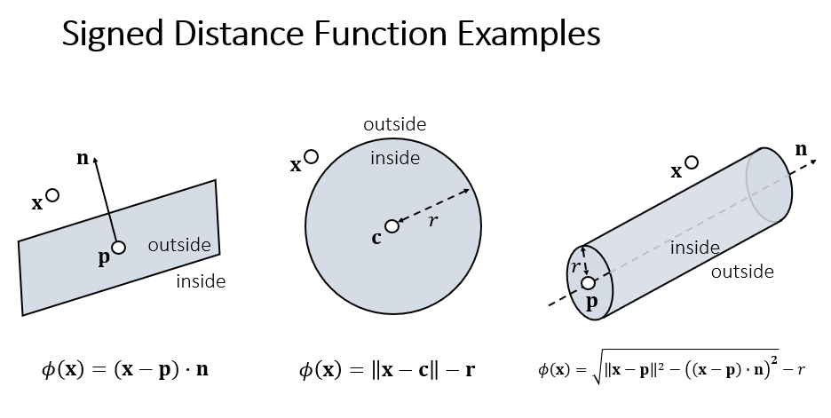
void Collision_Handling(){Mesh mesh = GetComponent<MeshFilter> ().mesh;Vector3[] X = mesh.vertices;//Handle colllision.Vector3 ballPos = GameObject.Find("Sphere").transform.position;float radius = 2.7f;for (int i = 0; i < X.Length; i++){if (i == 0 || i == 20) continue;if (SDF(X[i], ballPos)){V[i] = V[i] + 1.0f / t * (ballPos + radius * (X[i] - ballPos).normalized - X[i]);X[i] = ballPos + radius * (X[i] - ballPos).normalized;}}}bool SDF(Vector3 v, Vector3 center, float radius = 2.7f){float sdf = (v - center).magnitude - radius;return sdf > 0.0f ? false : true;}
Once a colliding vertex is found, apply impulse-based method as follows:
\]
图片来源:Games103
Cloth Simulation with Root Finding and Optimization的更多相关文章
- [zz] Pixar’s OpenSubdiv V2: A detailed look
http://www.fxguide.com/featured/pixars-opensubdiv-v2-a-detailed-look/ Pixar’s OpenSubdiv V2: A detai ...
- My Open Source Projects
• MyMagicBox (https://github.com/yaoyansi/mymagicbox) Role: Creator Miscellaneous projects for e ...
- Computer Graphics Research Software
Computer Graphics Research Software Helping you avoid re-inventing the wheel since 2009! Last update ...
- Matlab 中S-函数的使用 sfuntmpl
function [sys,x0,str,ts,simStateCompliance] = sfuntmpl(t,x,u,flag) %SFUNTMPL General MATLAB S-Functi ...
- Optimizing graphics performance
看U3D文档,心得:对于3D场景,使用分层次的距离裁剪,小物件分到一个层,稍远时就被裁掉,大物体分到一个层,距离很远时才裁掉,甚至不载.中物体介于二者之间. 文档如下: Good performanc ...
- Code Project精彩系列(转)
Code Project精彩系列(转) Code Project精彩系列(转) Applications Crafting a C# forms Editor From scratch htt ...
- 万字教你如何用 Python 实现线性规划
摘要:线性规划是一组数学和计算工具,可让您找到该系统的特定解,该解对应于某些其他线性函数的最大值或最小值. 本文分享自华为云社区<实践线性规划:使用 Python 进行优化>,作者: Yu ...
- Position Based Dynamics【译】
绝大部分机翻,少部分手动矫正,仅供参考.本人水平有限,如有误翻,概不负责... Position Based Dynamics Abstract The most popular approaches ...
- 网格弹簧质点系统模拟(Spring-Mass System by Euler Integration)
弹簧质点模型是利用牛顿运动定律来模拟物体变形的方法.如下图所示,该模型是一个由m×n个虚拟质点组成的网格,质点之间用无质量的.自然长度不为零的弹簧连接.其连接关系有以下三种: 1.连接质点[i, j] ...
- 编写更少量的代码:使用apache commons工具类库
Commons-configuration Commons-FileUpload Commons DbUtils Commons BeanUtils Commons CLI Commo ...
随机推荐
- Linux系统下使用pytorch多进程读取图片数据时的注意事项——DataLoader的多进程使用注意事项
原文: PEP 703 – Making the Global Interpreter Lock Optional in CPython 相关内容: The GIL Affects Python Li ...
- 说说中国高校理工科教育中的基础概念混乱问题——GPU是ASIC吗
在YouTube上看到这样一个视频: https://www.youtube.com/watch?v=7EXDp6c9n-Q&lc=Ugydwl8gppB5FWE8Y5V4AaABAg.9fc ...
- CH04_程序流程结构
CH04_程序流程结构 程序流程结构 C/C++支持最基本的三种程序运行结构: 顺序结构:程序按顺序执行,不发生挑战 选择结构:依据条件是否满足,有选择的执行相应的功能 循环结构:依据条件是否满足,循 ...
- 5 个有趣的 Python 开源项目「GitHub 热点速览」
本期,我从上周的开源热搜项目中精心挑选了 5 个有趣.好玩的 Python 开源项目. 首先是 PyScript,它可以让你直接在浏览器中运行 Python 代码,不仅支持在 HTML 中嵌入,还能安 ...
- 金融、支付行业的开发者不得不知道的float、double计算误差问题
为什么浮点数 float 或 double 运算的时候会有精度丢失的风险呢? <阿里巴巴 Java 开发手册>中提到:"浮点数之间的等值判断,基本数据类型不能用 == 来比较,包 ...
- Tesla 开发者 API 指南:BLE 密钥 – 身份验证和车辆命令
注意:本工具只能运行于 mac 或者 linux, win下不支持. 1. 克隆项目到本地 https://github.com/teslamotors/vehicle-command.git 2. ...
- mysql外键设置失败踩坑记录
把表里面的数据清空再添加 原因 因为外键一定要对应外面那个表的数据,现在添加外键会导致这个外键的值为空,违反了键的非空约定 理解为已有的数据突然多出来个字段,但是不知道值是什么,那就为空了 主键和外键 ...
- Linux 常见编辑器
命令行编辑器 Vim Linux 上最出名的编辑器当属 Vim 了.Vim 由 Vi 发展而来,Vim 的名字意指 Vi IMproved,表示 Vi 的升级版.Vim 对于新手来说使用比较复杂,不过 ...
- [深度学习] 时间序列分析工具TSLiB库使用指北
TSLiB是一个为深度学习时间序列分析量身打造的开源仓库.它提供了多种深度时间序列模型的统一实现,方便研究人员评估现有模型或开发定制模型.TSLiB涵盖了长时预测(Long-term forecast ...
- webpack系列-externals配置使用(CDN方式引入JS)
如果需要引用一个库,但是又不想让webpack打包(减少打包的时间),并且又不影响我们在程序中以CMD.AMD或者window/global全局等方式进行使用(一般都以import方式引用使用),那就 ...