惊不惊喜, 用深度学习 把设计图 自动生成HTML代码 !
如何用前端页面原型生成对应的代码一直是我们关注的问题,本文作者根据 pix2code 等论文构建了一个强大的前端代码生成模型,并详细解释了如何利用 LSTM 与 CNN 将设计原型编写为 HTML 和 CSS 网站。
项目链接:https://github.com/emilwallner/Screenshot-to-code-in-Keras
在未来三年内,深度学习将改变前端开发。它将会加快原型设计速度,拉低开发软件的门槛。
Tony Beltramelli 在去年发布了论文《pix2code: Generating Code from a Graphical User Interface Screenshot》,Airbnb 也发布了 Sketch2code(https://airbnb.design/sketching-interfaces/)。
目前,自动化前端开发的最大阻碍是计算能力。但我们已经可以使用目前的深度学习算法,以及合成训练数据来探索人工智能自动构建前端的方法。在本文中,作者将教神经网络学习基于一张图片和一个设计模板来编写一个 HTML 和 CSS 网站。以下是该过程的简要概述:
1)向训练过的神经网络输入一个设计图
2)神经网络将图片转化为 HTML 标记语言
3)渲染输出

我们将分三步从易到难构建三个不同的模型,首先,我们构建最简单地版本来掌握移动部件。第二个版本 HTML 专注于自动化所有步骤,并简要解释神经网络层。在最后一个版本 Bootstrap 中,我们将创建一个模型来思考和探索 LSTM 层。
代码地址:
- https://github.com/emilwallner/Screenshot-to-code-in-Keras
- https://www.floydhub.com/emilwallner/projects/picturetocode
所有 FloydHub notebook 都在 floydhub 目录中,本地 notebook 在 local 目录中。
本文中的模型构建基于 Beltramelli 的论文《pix2code: Generating Code from a Graphical User Interface Screenshot》和 Jason Brownlee 的图像描述生成教程,并使用 Python 和 Keras 完成。
核心逻辑
我们的目标是构建一个神经网络,能够生成与截图对应的 HTML/CSS 标记语言。
训练神经网络时,你先提供几个截图和对应的 HTML 代码。网络通过逐个预测所有匹配的 HTML 标记语言来学习。预测下一个标记语言的标签时,网络接收到截图和之前所有正确的标记。
这里是一个简单的训练数据示例:https://docs.google.com/spreadsheets/d/1xXwarcQZAHluorveZsACtXRdmNFbwGtN3WMNhcTdEyQ/edit?usp=sharing。
创建逐词预测的模型是现在最常用的方法,也是本教程使用的方法。
注意:每次预测时,神经网络接收的是同样的截图。也就是说如果网络需要预测 20 个单词,它就会得到 20 次同样的设计截图。现在,不用管神经网络的工作原理,只需要专注于神经网络的输入和输出。

我们先来看前面的标记(markup)。假如我们训练神经网络的目的是预测句子「I can code」。当网络接收「I」时,预测「can」。下一次时,网络接收「I can」,预测「code」。它接收所有之前单词,但只预测下一个单词。
神经网络根据数据创建特征。神经网络构建特征以连接输入数据和输出数据。它必须创建表征来理解每个截图的内容和它所需要预测的 HTML 语法,这些都是为预测下一个标记构建知识。把训练好的模型应用到真实世界中和模型训练过程差不多。
我们无需输入正确的 HTML 标记,网络会接收它目前生成的标记,然后预测下一个标记。预测从「起始标签」(start tag)开始,到「结束标签」(end tag)终止,或者达到最大限制时终止。

Hello World 版
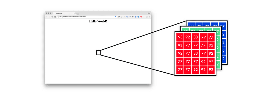
现在让我们构建 Hello World 版实现。我们将馈送一张带有「Hello World!」字样的截屏到神经网络中,并训练它生成对应的标记语言。
首先,神经网络将原型设计转换为一组像素值。且每一个像素点有 RGB 三个通道,每个通道的值都在 0-255 之间。
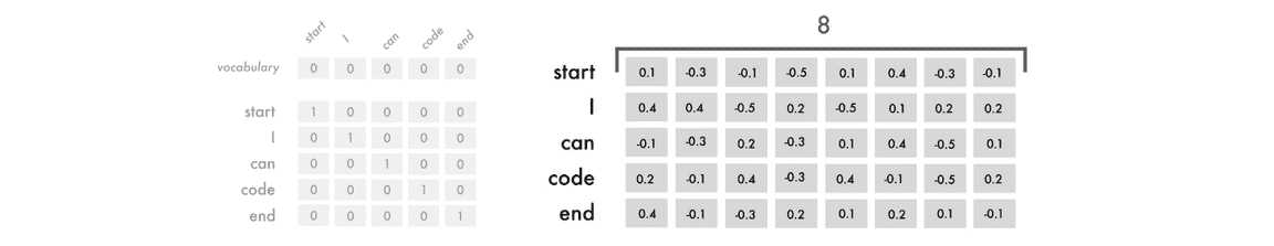
为了以神经网络能理解的方式表征这些标记,我使用了 one-hot 编码。因此句子「I can code」可以映射为以下形式。
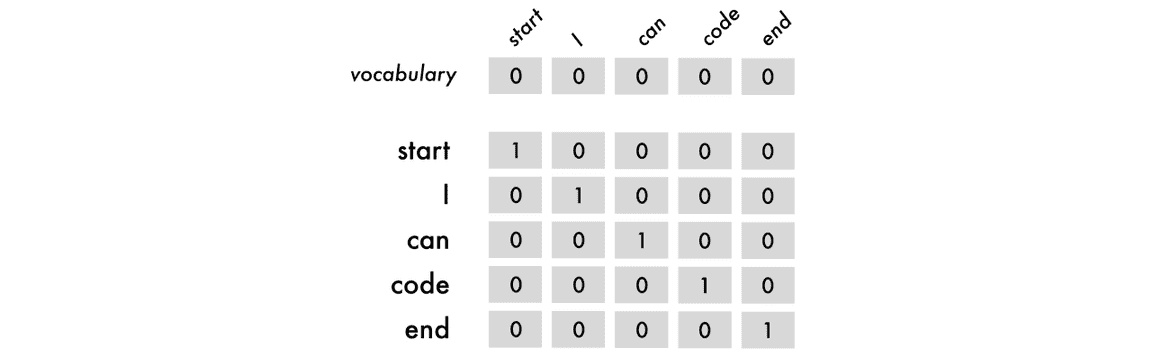
在上图中,我们的编码包含了开始和结束的标签。这些标签能为神经网络提供开始预测和结束预测的位置信息。以下是这些标签的各种组合以及对应 one-hot 编码的情况。

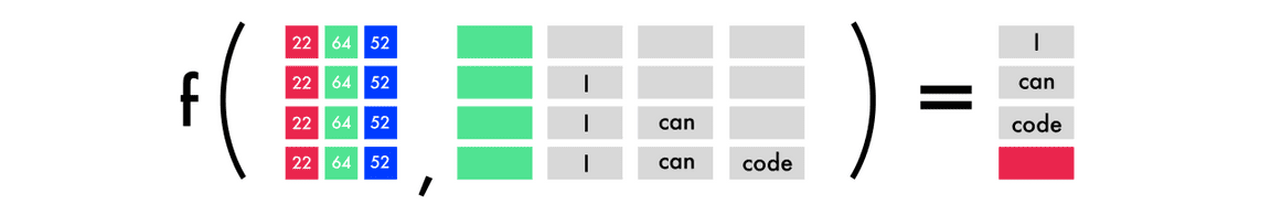
我们会使每个单词在每一轮训练中改变位置,因此这允许模型学习序列而不是记忆词的位置。在下图中有四个预测,每一行是一个预测。且左边代表 RGB 三色通道和之前的词,右边代表预测结果和红色的结束标签。
- #Length of longest sentence
- max_caption_len = 3
- #Size of vocabulary
- vocab_size = 3
- # Load one screenshot for each word and turn them into digits
- images = []
- for i in range(2):
- images.append(img_to_array(load_img('screenshot.jpg', target_size=(224, 224))))
- images = np.array(images, dtype=float)
- # Preprocess input for the VGG16 model
- images = preprocess_input(images)
- #Turn start tokens into one-hot encoding
- html_input = np.array(
- [[[0., 0., 0.], #start
- [0., 0., 0.],
- [1., 0., 0.]],
- [[0., 0., 0.], #start <HTML>Hello World!</HTML>
- [1., 0., 0.],
- [0., 1., 0.]]])
- #Turn next word into one-hot encoding
- next_words = np.array(
- [[0., 1., 0.], # <HTML>Hello World!</HTML>
- [0., 0., 1.]]) # end
- # Load the VGG16 model trained on imagenet and output the classification feature
- VGG = VGG16(weights='imagenet', include_top=True)
- # Extract the features from the image
- features = VGG.predict(images)
- #Load the feature to the network, apply a dense layer, and repeat the vector
- vgg_feature = Input(shape=(1000,))
- vgg_feature_dense = Dense(5)(vgg_feature)
- vgg_feature_repeat = RepeatVector(max_caption_len)(vgg_feature_dense)
- # Extract information from the input seqence
- language_input = Input(shape=(vocab_size, vocab_size))
- language_model = LSTM(5, return_sequences=True)(language_input)
- # Concatenate the information from the image and the input
- decoder = concatenate([vgg_feature_repeat, language_model])
- # Extract information from the concatenated output
- decoder = LSTM(5, return_sequences=False)(decoder)
- # Predict which word comes next
- decoder_output = Dense(vocab_size, activation='softmax')(decoder)
- # Compile and run the neural network
- model = Model(inputs=[vgg_feature, language_input], outputs=decoder_output)
- model.compile(loss='categorical_crossentropy', optimizer='rmsprop')
- # Train the neural network
- model.fit([features, html_input], next_words, batch_size=2, shuffle=False, epochs=1000)
在 Hello World 版本中,我们使用三个符号「start」、「Hello World」和「end」。字符级的模型要求更小的词汇表和受限的神经网络,而单词级的符号在这里可能有更好的性能。
以下是执行预测的代码:
- # Create an empty sentence and insert the start token
- sentence = np.zeros((1, 3, 3)) # [[0,0,0], [0,0,0], [0,0,0]]
- start_token = [1., 0., 0.] # start
- sentence[0][2] = start_token # place start in empty sentence
- # Making the first prediction with the start token
- second_word = model.predict([np.array([features[1]]), sentence])
- # Put the second word in the sentence and make the final prediction
- sentence[0][1] = start_token
- sentence[0][2] = np.round(second_word)
- third_word = model.predict([np.array([features[1]]), sentence])
- # Place the start token and our two predictions in the sentence
- sentence[0][0] = start_token
- sentence[0][1] = np.round(second_word)
- sentence[0][2] = np.round(third_word)
- # Transform our one-hot predictions into the final tokens
- vocabulary = ["start", "<HTML><center><H1>Hello World!</H1></center></HTML>", "end"]
- for i in sentence[0]:
- print(vocabulary[np.argmax(i)], end=' ')
输出
- 10 epochs: start start start
- 100 epochs: start <HTML><center><H1>Hello World!</H1></center></HTML> <HTML><center><H1>Hello World!</H1></center></HTML>
- 300 epochs: start <HTML><center><H1>Hello World!</H1></center></HTML> end
我走过的坑:
- 在收集数据之前构建第一个版本。在本项目的早期阶段,我设法获得 Geocities 托管网站的旧版存档,它有 3800 万的网站。但我忽略了减少 100K 大小词汇所需要的巨大工作量。
- 训练一个 TB 级的数据需要优秀的硬件或极其有耐心。在我的 Mac 遇到几个问题后,最终用上了强大的远程服务器。我预计租用 8 个现代 CPU 和 1 GPS 内部链接以运行我的工作流。
- 在理解输入与输出数据之前,其它部分都似懂非懂。输入 X 是屏幕的截图和以前标记的标签,输出 Y 是下一个标记的标签。当我理解这一点时,其它问题都更加容易弄清了。此外,尝试其它不同的架构也将更加容易。
- 图片到代码的网络其实就是自动描述图像的模型。即使我意识到了这一点,但仍然错过了很多自动图像摘要方面的论文,因为它们看起来不够炫酷。一旦我意识到了这一点,我对问题空间的理解就变得更加深刻了。
在 FloydHub 上运行代码
FloydHub 是一个深度学习训练平台,我自从开始学习深度学习时就对它有所了解,我也常用它训练和管理深度学习试验。我们能安装它并在 10 分钟内运行第一个模型,它是在云 GPU 上训练模型最好的选择。若果读者没用过 FloydHub,可以花 10 分钟左右安装并了解。
FloydHub 地址:https://www.floydhub.com/
复制 Repo:
- https://github.com/emilwallner/Screenshot-to-code-in-Keras.git
登录并初始化 FloydHub 命令行工具:
- cd Screenshot-to-code-in-Keras
- floyd login
- floyd init s2c
在 FloydHub 云 GPU 机器上运行 Jupyter notebook:
- floyd run --gpu --env tensorflow-1.4 --data emilwallner/datasets/imagetocode/2:data --mode jupyter
所有的 notebook 都放在 floydbub 目录下。一旦我们开始运行模型,那么在 floydhub/Helloworld/helloworld.ipynb 下可以找到第一个 Notebook。更多详情请查看本项目早期的 flags。
HTML 版本
在这个版本中,我们将关注与创建一个可扩展的神经网络模型。该版本并不能直接从随机网页预测 HTML,但它是探索动态问题不可缺少的步骤。
概览
如果我们将前面的架构扩展为以下右图展示的结构,那么它就能更高效地处理识别与转换过程。
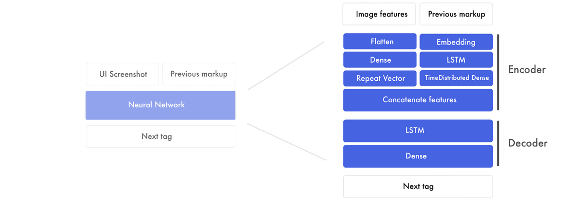
该架构主要有两个部,即编码器与解码器。编码器是我们创建图像特征和前面标记特征(markup features)的部分。特征是网络创建原型设计和标记语言之间联系的构建块。在编码器的末尾,我们将图像特征传递给前面标记的每一个单词。随后解码器将结合原型设计特征和标记特征以创建下一个标签的特征,这一个特征可以通过全连接层预测下一个标签。
设计原型的特征
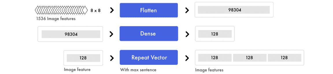
因为我们需要为每个单词插入一个截屏,这将会成为训练神经网络的瓶颈。因此我们抽取生成标记语言所需要的信息来替代直接使用图像。这些抽取的信息将通过预训练的 CNN 编码到图像特征中,且我们将使用分类层之前的层级输出以抽取特征。

我们最终得到 1536 个 8*8 的特征图,虽然我们很难直观地理解它,但神经网络能够从这些特征中抽取元素的对象和位置。
标记特征
在 Hello World 版本中,我们使用 one-hot 编码以表征标记。而在该版本中,我们将使用词嵌入表征输入并使用 one-hot 编码表示输出。我们构建每个句子的方式保持不变,但我们映射每个符号的方式将会变化。one-hot 编码将每一个词视为独立的单元,而词嵌入会将输入数据表征为一个实数列表,这些实数表示标记标签之间的关系。
上面词嵌入的维度为 8,但一般词嵌入的维度会根据词汇表的大小在 50 到 500 间变动。以上每个单词的八个数值就类似于神经网络中的权重,它们倾向于刻画单词之间的联系(Mikolov alt el., 2013)。这就是我们开始部署标记特征(markup features)的方式,而这些神经网络训练的特征会将输入数据和输出数据联系起来。
编码器
我们现在将词嵌入馈送到 LSTM 中,并期望能返回一系列的标记特征。这些标记特征随后会馈送到一个 Time Distributed 密集层,该层级可以视为有多个输入和输出的全连接层。
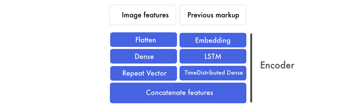
和嵌入与 LSTM 层相平行的还有另外一个处理过程,其中图像特征首先会展开成一个向量,然后再馈送到一个全连接层而抽取出高级特征。这些图像特征随后会与标记特征相级联而作为编码器的输出。
标记特征
如下图所示,现在我们将词嵌入投入到 LSTM 层中,所有的语句都会用零填充以获得相同的向量长度。

为了混合信号并寻找高级模式,我们运用了一个 TimeDistributed 密集层以抽取标记特征。TimeDistributed 密集层和一般的全连接层非常相似,且它有多个输入与输出。
图像特征
对于另一个平行的过程,我们需要将图像的所有像素值展开成一个向量,因此信息不会被改变,它们只会用来识别。
如上,我们会通过全连接层混合信号并抽取更高级的概念。因为我们并不只是处理一个输入值,因此使用一般的全连接层就行了。
级联图像特征和标记特征
所有的语句都被填充以创建三个标记特征。因为我们已经预处理了图像特征,所以我们能为每一个标记特征添加图像特征。
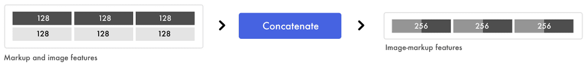
如上,在复制图像特征到对应的标记特征后,我们得到了新的图像-标记特征(image-markup features),这就是我们馈送到解码器的输入值。
解码器
现在,我们使用图像-标记特征来预测下一个标签。

在下面的案例中,我们使用三个图像-标签特征对来输出下一个标签特征。注意 LSTM 层不应该返回一个长度等于输入序列的向量,而只需要预测预测一个特征。在我们的案例中,这个特征将预测下一个标签,它包含了最后预测的信息。
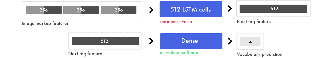
最后的预测
密集层会像传统前馈网络那样工作,它将下一个标签特征中的 512 个值与最后的四个预测连接起来,即我们在词汇表所拥有的四个单词:start、hello、world 和 end。密集层最后采用的 softmax 函数会为四个类别产生一个概率分布,例如 [0.1, 0.1, 0.1, 0.7] 将预测第四个词为下一个标签。
- # Load the images and preprocess them for inception-resnet
- images = []
- all_filenames = listdir('images/')
- all_filenames.sort()
- for filename in all_filenames:
- images.append(img_to_array(load_img('images/'+filename, target_size=(299, 299))))
- images = np.array(images, dtype=float)
- images = preprocess_input(images)
- # Run the images through inception-resnet and extract the features without the classification layer
- IR2 = InceptionResNetV2(weights='imagenet', include_top=False)
- features = IR2.predict(images)
- # We will cap each input sequence to 100 tokens
- max_caption_len = 100
- # Initialize the function that will create our vocabulary
- tokenizer = Tokenizer(filters='', split=" ", lower=False)
- # Read a document and return a string
- def load_doc(filename):
- file = open(filename, 'r')
- text = file.read()
- file.close()
- return text
- # Load all the HTML files
- X = []
- all_filenames = listdir('html/')
- all_filenames.sort()
- for filename in all_filenames:
- X.append(load_doc('html/'+filename))
- # Create the vocabulary from the html files
- tokenizer.fit_on_texts(X)
- # Add +1 to leave space for empty words
- vocab_size = len(tokenizer.word_index) + 1
- # Translate each word in text file to the matching vocabulary index
- sequences = tokenizer.texts_to_sequences(X)
- # The longest HTML file
- max_length = max(len(s) for s in sequences)
- # Intialize our final input to the model
- X, y, image_data = list(), list(), list()
- for img_no, seq in enumerate(sequences):
- for i in range(1, len(seq)):
- # Add the entire sequence to the input and only keep the next word for the output
- in_seq, out_seq = seq[:i], seq[i]
- # If the sentence is shorter than max_length, fill it up with empty words
- in_seq = pad_sequences([in_seq], maxlen=max_length)[0]
- # Map the output to one-hot encoding
- out_seq = to_categorical([out_seq], num_classes=vocab_size)[0]
- # Add and image corresponding to the HTML file
- image_data.append(features[img_no])
- # Cut the input sentence to 100 tokens, and add it to the input data
- X.append(in_seq[-100:])
- y.append(out_seq)
- X, y, image_data = np.array(X), np.array(y), np.array(image_data)
- # Create the encoder
- image_features = Input(shape=(8, 8, 1536,))
- image_flat = Flatten()(image_features)
- image_flat = Dense(128, activation='relu')(image_flat)
- ir2_out = RepeatVector(max_caption_len)(image_flat)
- language_input = Input(shape=(max_caption_len,))
- language_model = Embedding(vocab_size, 200, input_length=max_caption_len)(language_input)
- language_model = LSTM(256, return_sequences=True)(language_model)
- language_model = LSTM(256, return_sequences=True)(language_model)
- language_model = TimeDistributed(Dense(128, activation='relu'))(language_model)
- # Create the decoder
- decoder = concatenate([ir2_out, language_model])
- decoder = LSTM(512, return_sequences=False)(decoder)
- decoder_output = Dense(vocab_size, activation='softmax')(decoder)
- # Compile the model
- model = Model(inputs=[image_features, language_input], outputs=decoder_output)
- model.compile(loss='categorical_crossentropy', optimizer='rmsprop')
- # Train the neural network
- model.fit([image_data, X], y, batch_size=64, shuffle=False, epochs=2)
- # map an integer to a word
- def word_for_id(integer, tokenizer):
- for word, index in tokenizer.word_index.items():
- if index == integer:
- return word
- return None
- # generate a deion for an image
- def generate_desc(model, tokenizer, photo, max_length):
- # seed the generation process
- in_text = 'START'
- # iterate over the whole length of the sequence
- for i in range(900):
- # integer encode input sequence
- sequence = tokenizer.texts_to_sequences([in_text])[0][-100:]
- # pad input
- sequence = pad_sequences([sequence], maxlen=max_length)
- # predict next word
- yhat = model.predict([photo,sequence], verbose=0)
- # convert probability to integer
- yhat = np.argmax(yhat)
- # map integer to word
- word = word_for_id(yhat, tokenizer)
- # stop if we cannot map the word
- if word is None:
- break
- # append as input for generating the next word
- in_text += ' ' + word
- # Print the prediction
- print(' ' + word, end='')
- # stop if we predict the end of the sequence
- if word == 'END':
- break
- return
- # Load and image, preprocess it for IR2, extract features and generate the HTML
- test_image = img_to_array(load_img('images/87.jpg', target_size=(299, 299)))
- test_image = np.array(test_image, dtype=float)
- test_image = preprocess_input(test_image)
- test_features = IR2.predict(np.array([test_image]))
- generate_desc(model, tokenizer, np.array(test_features), 100)
输出
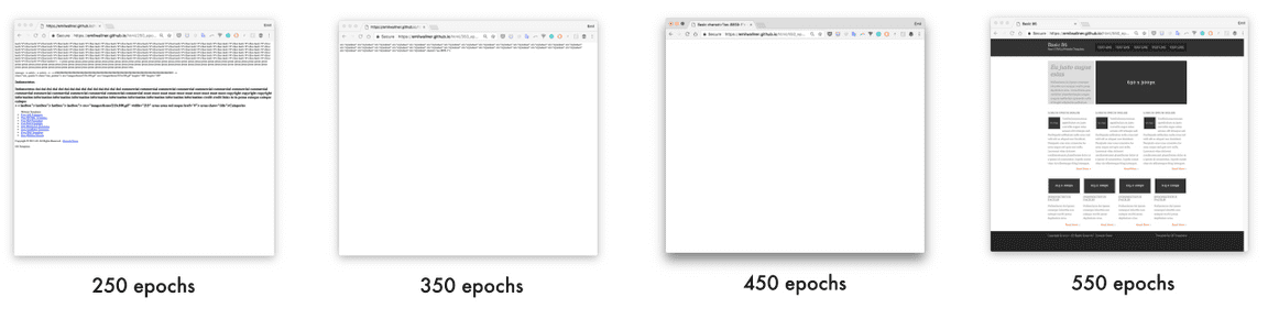
训练不同轮数所生成网站的地址:
- 250 epochs:https://emilwallner.github.io/html/250_epochs/
- 350 epochs:https://emilwallner.github.io/html/350_epochs/
- 450 epochs:https://emilwallner.github.io/html/450_epochs/
- 550 epochs:https://emilwallner.github.io/html/550_epochs/
我走过的坑:
- 我认为理解 LSTM 比 CNN 要难一些。当我展开 LSTM 后,它们会变得容易理解一些。此外,我们在尝试理解 LSTM 前,可以先关注输入与输出特征。
- 从头构建一个词汇表要比压缩一个巨大的词汇表容易得多。这样的构建包括字体、div 标签大小、变量名的 hex 颜色和一般单词。
- 大多数库是为解析文本文档而构建。在库的使用文档中,它们会告诉我们如何通过空格进行分割,而不是代码,我们需要自定义解析的方式。
- 我们可以从 ImageNet 上预训练的模型抽取特征。然而,相对于从头训练的 pix2code 模型,损失要高 30% 左右。此外,我对于使用基于网页截屏预训练的 inception-resnet 网络很有兴趣。
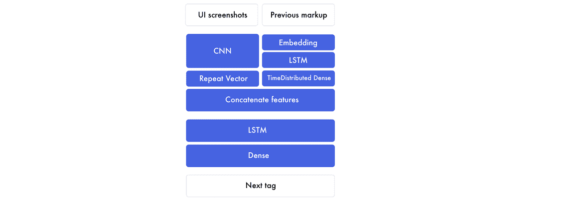
Bootstrap 版本
在最终版本中,我们使用 pix2code 论文中生成 bootstrap 网站的数据集。使用 Twitter 的 Bootstrap 库(https://getbootstrap.com/),我们可以结合 HTML 和 CSS,降低词汇表规模。
我们将使用这一版本为之前未见过的截图生成标记。我们还深入研究它如何构建截图和标记的先验知识。
我们不在 bootstrap 标记上训练,而是使用 17 个简化 token,将其编译成 HTML 和 CSS。数据集(https://github.com/tonybeltramelli/pix2code/tree/master/datasets)包括 1500 个测试截图和 250 个验证截图。平均每个截图有 65 个 token,一共有 96925 个训练样本。
我们稍微修改一下 pix2code 论文中的模型,使之预测网络组件的准确率达到 97%。
端到端方法
从预训练模型中提取特征在图像描述生成模型中效果很好。但是几次实验后,我发现 pix2code 的端到端方法效果更好。在我们的模型中,我们用轻量级卷积神经网络替换预训练图像特征。我们不使用最大池化来增加信息密度,而是增加步幅。这可以保持前端元素的位置和颜色。
存在两个核心模型:卷积神经网络(CNN)和循环神经网络(RNN)。最常用的循环神经网络是长短期记忆(LSTM)网络。我之前的文章中介绍过 CNN 教程,本文主要介绍 LSTM。
理解 LSTM 中的时间步
关于 LSTM 比较难理解的是时间步。我们的原始神经网络有两个时间步,如果你给它「Hello」,它就会预测「World」。但是它会试图预测更多时间步。下例中,输入有四个时间步,每个单词对应一个时间步。
LSTM 适合时序数据的输入,它是一种适合顺序信息的神经网络。模型展开图示如下,对于每个循环步,你需要保持同样的权重。
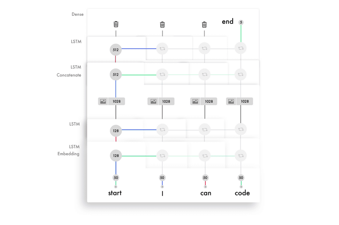
加权后的输入与输出特征在级联后输入到激活函数,并作为当前时间步的输出。因为我们重复利用了相同的权重,它们将从一些输入获取信息并构建序列的知识。下面是 LSTM 在每一个时间步上的简化版处理过程:

理解 LSTM 层级中的单元
每一层 LSTM 单元的总数决定了它记忆的能力,同样也对应于每一个输出特征的维度大小。LSTM 层级中的每一个单元将学习如何追踪句法的不同方面。以下是一个 LSTM 单元追踪标签行信息的可视化,它是我们用来训练 bootstrap 模型的简单标记语言。
每一个 LSTM 单元会维持一个单元状态,我们可以将单元状态视为记忆。权重和激活值可使用不同的方式修正状态值,这令 LSTM 层可以通过保留或遗忘输入信息而得到精调。除了处理当前输入信息与输出信息,LSTM 单元还需要修正记忆状态以传递到下一个时间步。
- dir_name = 'resources/eval_light/'
- # Read a file and return a string
- def load_doc(filename):
- file = open(filename, 'r')
- text = file.read()
- file.close()
- return text
- def load_data(data_dir):
- text = []
- images = []
- # Load all the files and order them
- all_filenames = listdir(data_dir)
- all_filenames.sort()
- for filename in (all_filenames):
- if filename[-3:] == "npz":
- # Load the images already prepared in arrays
- image = np.load(data_dir+filename)
- images.append(image['features'])
- else:
- # Load the boostrap tokens and rap them in a start and end tag
- syntax = '<START> ' + load_doc(data_dir+filename) + ' <END>'
- # Seperate all the words with a single space
- syntax = ' '.join(syntax.split())
- # Add a space after each comma
- syntax = syntax.replace(',', ' ,')
- text.append(syntax)
- images = np.array(images, dtype=float)
- return images, text
- train_features, texts = load_data(dir_name)
- # Initialize the function to create the vocabulary
- tokenizer = Tokenizer(filters='', split=" ", lower=False)
- # Create the vocabulary
- tokenizer.fit_on_texts([load_doc('bootstrap.vocab')])
- # Add one spot for the empty word in the vocabulary
- vocab_size = len(tokenizer.word_index) + 1
- # Map the input sentences into the vocabulary indexes
- train_sequences = tokenizer.texts_to_sequences(texts)
- # The longest set of boostrap tokens
- max_sequence = max(len(s) for s in train_sequences)
- # Specify how many tokens to have in each input sentence
- max_length = 48
- def preprocess_data(sequences, features):
- X, y, image_data = list(), list(), list()
- for img_no, seq in enumerate(sequences):
- for i in range(1, len(seq)):
- # Add the sentence until the current count(i) and add the current count to the output
- in_seq, out_seq = seq[:i], seq[i]
- # Pad all the input token sentences to max_sequence
- in_seq = pad_sequences([in_seq], maxlen=max_sequence)[0]
- # Turn the output into one-hot encoding
- out_seq = to_categorical([out_seq], num_classes=vocab_size)[0]
- # Add the corresponding image to the boostrap token file
- image_data.append(features[img_no])
- # Cap the input sentence to 48 tokens and add it
- X.append(in_seq[-48:])
- y.append(out_seq)
- return np.array(X), np.array(y), np.array(image_data)
- X, y, image_data = preprocess_data(train_sequences, train_features)
- #Create the encoder
- image_model = Sequential()
- image_model.add(Conv2D(16, (3, 3), padding='valid', activation='relu', input_shape=(256, 256, 3,)))
- image_model.add(Conv2D(16, (3,3), activation='relu', padding='same', strides=2))
- image_model.add(Conv2D(32, (3,3), activation='relu', padding='same'))
- image_model.add(Conv2D(32, (3,3), activation='relu', padding='same', strides=2))
- image_model.add(Conv2D(64, (3,3), activation='relu', padding='same'))
- image_model.add(Conv2D(64, (3,3), activation='relu', padding='same', strides=2))
- image_model.add(Conv2D(128, (3,3), activation='relu', padding='same'))
- image_model.add(Flatten())
- image_model.add(Dense(1024, activation='relu'))
- image_model.add(Dropout(0.3))
- image_model.add(Dense(1024, activation='relu'))
- image_model.add(Dropout(0.3))
- image_model.add(RepeatVector(max_length))
- visual_input = Input(shape=(256, 256, 3,))
- encoded_image = image_model(visual_input)
- language_input = Input(shape=(max_length,))
- language_model = Embedding(vocab_size, 50, input_length=max_length, mask_zero=True)(language_input)
- language_model = LSTM(128, return_sequences=True)(language_model)
- language_model = LSTM(128, return_sequences=True)(language_model)
- #Create the decoder
- decoder = concatenate([encoded_image, language_model])
- decoder = LSTM(512, return_sequences=True)(decoder)
- decoder = LSTM(512, return_sequences=False)(decoder)
- decoder = Dense(vocab_size, activation='softmax')(decoder)
- # Compile the model
- model = Model(inputs=[visual_input, language_input], outputs=decoder)
- optimizer = RMSprop(lr=0.0001, clipvalue=1.0)
- model.compile(loss='categorical_crossentropy', optimizer=optimizer)
- #Save the model for every 2nd epoch
- filepath="org-weights-epoch-{epoch:04d}--val_loss-{val_loss:.4f}--loss-{loss:.4f}.hdf5"
- checkpoint = ModelCheckpoint(filepath, monitor='val_loss', verbose=1, save_weights_only=True, period=2)
- callbacks_list = [checkpoint]
- # Train the model
- model.fit([image_data, X], y, batch_size=64, shuffle=False, validation_split=0.1, callbacks=callbacks_list, verbose=1, epochs=50)
测试准确率
找到一种测量准确率的优秀方法非常棘手。比如一个词一个词地对比,如果你的预测中有一个词不对照,准确率可能就是 0。如果你把百分百对照的单词移除一个,最终的准确率可能是 99/100。
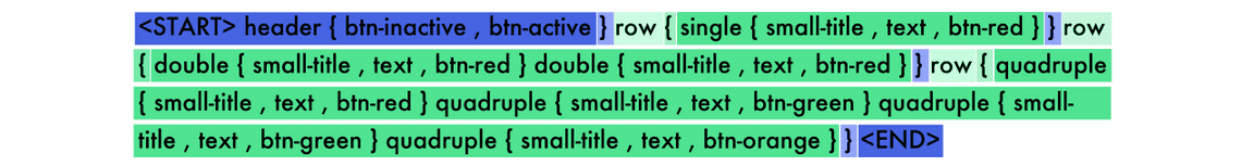
我使用的是 BLEU 分值,它在机器翻译和图像描述模型实践上都是最好的。它把句子分解成 4 个 n-gram,从 1-4 个单词的序列。在下面的预测中,「cat」应该是「code」。

为了得到最终的分值,每个的分值需要乘以 25%,(4/5) × 0.25 + (2/4) × 0.25 + (1/3) ×0.25 + (0/2) ×0.25 = 0.2 + 0.125 + 0.083 + 0 = 0.408。然后用总和乘以句子长度的惩罚函数。因为在我们的示例中,长度是正确的,所以它就直接是我们的最终得分。
你可以增加 n-gram 的数量,4 个 n-gram 的模型是最为对应人类翻译的。我建议你阅读下面的代码:
- #Create a function to read a file and return its content
- def load_doc(filename):
- file = open(filename, 'r')
- text = file.read()
- file.close()
- return text
- def load_data(data_dir):
- text = []
- images = []
- files_in_folder = os.listdir(data_dir)
- files_in_folder.sort()
- for filename in tqdm(files_in_folder):
- #Add an image
- if filename[-3:] == "npz":
- image = np.load(data_dir+filename)
- images.append(image['features'])
- else:
- # Add text and wrap it in a start and end tag
- syntax = '<START> ' + load_doc(data_dir+filename) + ' <END>'
- #Seperate each word with a space
- syntax = ' '.join(syntax.split())
- #Add a space between each comma
- syntax = syntax.replace(',', ' ,')
- text.append(syntax)
- images = np.array(images, dtype=float)
- return images, text
- #Intialize the function to create the vocabulary
- tokenizer = Tokenizer(filters='', split=" ", lower=False)
- #Create the vocabulary in a specific order
- tokenizer.fit_on_texts([load_doc('bootstrap.vocab')])
- dir_name = '../../../../eval/'
- train_features, texts = load_data(dir_name)
- #load model and weights
- json_file = open('../../../../model.json', 'r')
- loaded_model_json = json_file.read()
- json_file.close()
- loaded_model = model_from_json(loaded_model_json)
- # load weights into new model
- loaded_model.load_weights("../../../../weights.hdf5")
- print("Loaded model from disk")
- # map an integer to a word
- def word_for_id(integer, tokenizer):
- for word, index in tokenizer.word_index.items():
- if index == integer:
- return word
- return None
- print(word_for_id(17, tokenizer))
- # generate a deion for an image
- def generate_desc(model, tokenizer, photo, max_length):
- photo = np.array([photo])
- # seed the generation process
- in_text = '<START> '
- # iterate over the whole length of the sequence
- print('nPrediction---->nn<START> ', end='')
- for i in range(150):
- # integer encode input sequence
- sequence = tokenizer.texts_to_sequences([in_text])[0]
- # pad input
- sequence = pad_sequences([sequence], maxlen=max_length)
- # predict next word
- yhat = loaded_model.predict([photo, sequence], verbose=0)
- # convert probability to integer
- yhat = argmax(yhat)
- # map integer to word
- word = word_for_id(yhat, tokenizer)
- # stop if we cannot map the word
- if word is None:
- break
- # append as input for generating the next word
- in_text += word + ' '
- # stop if we predict the end of the sequence
- print(word + ' ', end='')
- if word == '<END>':
- break
- return in_text
- max_length = 48
- # evaluate the skill of the model
- def evaluate_model(model, deions, photos, tokenizer, max_length):
- actual, predicted = list(), list()
- # step over the whole set
- for i in range(len(texts)):
- yhat = generate_desc(model, tokenizer, photos[i], max_length)
- # store actual and predicted
- print('nnReal---->nn' + texts[i])
- actual.append([texts[i].split()])
- predicted.append(yhat.split())
- # calculate BLEU score
- bleu = corpus_bleu(actual, predicted)
- return bleu, actual, predicted
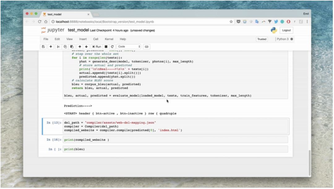
- bleu, actual, predicted = evaluate_model(loaded_model, texts, train_features, tokenizer, max_length)
- #Compile the tokens into HTML and css
- dsl_path = "compiler/assets/web-dsl-mapping.json"
- compiler = Compiler(dsl_path)
- compiled_website = compiler.compile(predicted[0], 'index.html')
- print(compiled_website )
- print(bleu)
输出
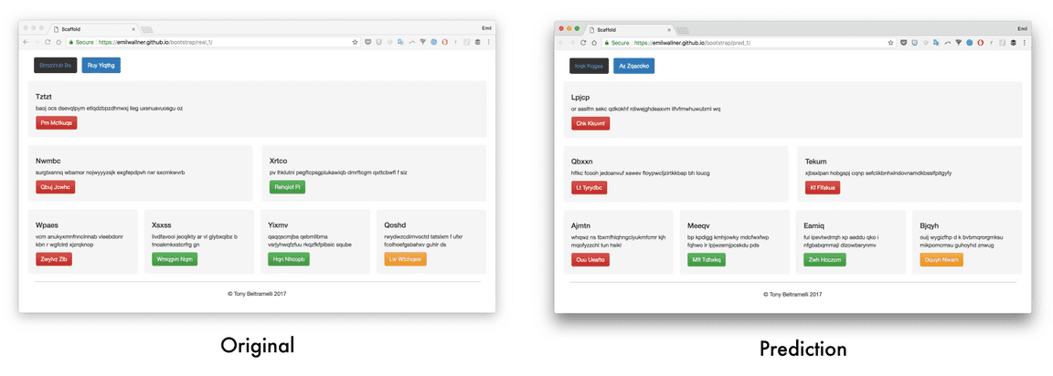
样本输出的链接:
- Generated website 1 - Original 1 (https://emilwallner.github.io/bootstrap/real_1/)
- Generated website 2 - Original 2 (https://emilwallner.github.io/bootstrap/real_2/)
- Generated website 3 - Original 3 (https://emilwallner.github.io/bootstrap/real_3/)
- Generated website 4 - Original 4 (https://emilwallner.github.io/bootstrap/real_4/)
- Generated website 5 - Original 5 (https://emilwallner.github.io/bootstrap/real_5/)
我走过的坑:
- 理解模型的弱点而不是测试随机模型。首先我使用随机的东西,比如批归一化、双向网络,并尝试实现注意力机制。在查看测试数据,并知道其无法高精度地预测颜色和位置之后,我意识到 CNN 存在一个弱点。这致使我使用增加的步幅来取代最大池化。验证损失从 0.12 降至 0.02,BLEU 分值从 85% 增加至 97%。
- 如果它们相关,则只使用预训练模型。在小数据的情况下,我认为一个预训练图像模型将会提升性能。从我的实验来看,端到端模型训练更慢,需要更多内存,但是精确度会提升 30%。
- 当你在远程服务器上运行模型,我们需要为一些不同做好准备。在我的 mac 上,它按照字母表顺序读取文档。但是在服务器上,它被随机定位。这在代码和截图之间造成了不匹配。
下一步
前端开发是深度学习应用的理想空间。数据容易生成,并且当前深度学习算法可以映射绝大部分逻辑。一个最让人激动的领域是注意力机制在 LSTM 上的应用。这不仅会提升精确度,还可以使我们可视化 CNN 在生成标记时所聚焦的地方。注意力同样是标记、可定义模板、脚本和最终端之间通信的关键。注意力层要追踪变量,使网络可以在编程语言之间保持通信。
但是在不久的将来,最大的影响将会来自合成数据的可扩展方法。接着你可以一步步添加字体、颜色和动画。目前为止,大多数进步发生在草图(sketches)方面并将其转化为模版应用。在不到两年的时间里,我们将创建一个草图,它会在一秒之内找到相应的前端。Airbnb 设计团队与 Uizard 已经创建了两个正在使用的原型。下面是一些可能的试验过程:
实验
开始
- 运行所有模型
- 尝试不同的超参数
- 测试一个不同的 CNN 架构
- 添加双向 LSTM 模型
- 用不同数据集实现模型
进一步实验返回搜狐,查看更多
- 使用相应的语法创建一个稳定的随机应用/网页生成器
- 从草图到应用模型的数据。自动将应用/网页截图转化为草图,并使用 GAN 创建多样性。
- 应用注意力层可视化每一预测的图像聚焦,类似于这个模型
- 为模块化方法创建一个框架。比如,有字体的编码器模型,一个用于颜色,另一个用于排版,并使用一个解码器整合它们。稳定的图像特征是一个好的开始。
- 馈送简单的 HTML 组件到神经网络中,并使用 CSS 教其生成动画。使用注意力方法并可视化两个输入源的聚焦将会很迷人。
惊不惊喜, 用深度学习 把设计图 自动生成HTML代码 !的更多相关文章
- 用深度学习技术FCN自动生成口红
1 这个是什么? 基于全卷积神经网络(FCN)的自动生成口红Python程序. 图1 FCN生成口红的效果(注:此两张人脸图来自人脸公开数据库LFW) 2 怎么使用了? 首 ...
- 深度学习之 rnn 台词生成
深度学习之 rnn 台词生成 写一个台词生成的程序,用 pytorch 写的. import os def load_data(path): with open(path, 'r', encoding ...
- 深度学习模型stacking模型融合python代码,看了你就会使
话不多说,直接上代码 def stacking_first(train, train_y, test): savepath = './stack_op{}_dt{}_tfidf{}/'.format( ...
- 深度学习框架如何自动选择最快的算法?Fast Run 让你收获最好的性能!
作者:王博文 | 旷视 MegEngine 架构师 一.背景 对于深度学习框架来说,网络的训练/推理时间是用户非常看中的.在实际生产条件下,用户设计的 NN 网络是千差万别,即使是同一类数学计算,参数 ...
- 基于深度学习的车辆检测系统(MATLAB代码,含GUI界面)
摘要:当前深度学习在目标检测领域的影响日益显著,本文主要基于深度学习的目标检测算法实现车辆检测,为大家介绍如何利用\(\color{#4285f4}{M}\color{#ea4335}{A}\colo ...
- 如何把设计图自动转换为iOS代码? 在线等,挺急的!
这是一篇可能略显枯燥的技术深度讨论与实践文章.如何把设计图自动转换为对应的iOS代码?作为一个 iOS开发爱好者,这是我很感兴趣的一个话题.最近也确实有了些许灵感,也确实取得了一点小成果,和大家分享一 ...
- Activiti工作流学习笔记(三)——自动生成28张数据库表的底层原理分析
原创/朱季谦 我接触工作流引擎Activiti已有两年之久,但一直都只限于熟悉其各类API的使用,对底层的实现,则存在较大的盲区. Activiti这个开源框架在设计上,其实存在不少值得学习和思考的地 ...
- 4.keras实现-->生成式深度学习之用GAN生成图像
生成式对抗网络(GAN,generative adversarial network)由Goodfellow等人于2014年提出,它可以替代VAE来学习图像的潜在空间.它能够迫使生成图像与真实图像在统 ...
- 【mybatis源码学习】利用maven插件自动生成mybatis代码
[一]在要生成代码的项目模块的pom.xml文件中添加maven插件 <!--mybatis代码生成器--> <plugin> <groupId>org.mybat ...
随机推荐
- Alyona and a tree CodeForces - 739B (线段树合并)
大意: 给定有根树, 每个点$x$有权值$a_x$, 对于每个点$x$, 求出$x$子树内所有点$y$, 需要满足$dist(x,y)<=a_y$. 刚开始想错了, 直接打线段树合并了..... ...
- phpunit——执行测试文件和测试文件中的某一个函数
phpunit --filter testDeleteFeed // 执行某一个测试函数 phpunit tests/Unit/Services/Feed/FeedLogTest.php // 执行某 ...
- Java对MongoDB中的数据查询处理
Java语言标准的数据库时MySQL,但是有些时候也会用到MongoDB,这次Boss交代处理MongoDB,所以讲代码以及思路记录下了 摸索的过程,才发现软件的适用还是很重要的啊!!! 我连接的Mo ...
- [python] 查找列表中重复的元素
a = [1, 2, 3, 2, 1, 5, 6, 5, 5, 5] b = set(a) for each_b in b: count = 0 for each_a in a: if each_b ...
- 通过selenium控制浏览器滚动条
目的:通过selenium控制浏览器滚动条 原理:通过 driver.execute_script()执行js代码,达到目的 driver.execute_script("window.sc ...
- 创建springboot的聚合工程(二)
前篇已经成功创建了springboot的聚合工程并成功访问,下面就要开始子工程木块之间的调用: springboot项目的特点,一个工程下面的类必须要放在启动类下面的子目录下面,否则,启动的时候会报错 ...
- CF-517C-思维/math
http://codeforces.com/contest/1072/problem/C 题目大意是给出两个数a,b ,找出若干个数p,使得 SUM{p}<=a ,找出若干个数q使得SUM{q} ...
- hdu-6437-最大费用流
Problem L.Videos Time Limit: 4000/2000 MS (Java/Others) Memory Limit: 524288/524288 K (Java/Other ...
- WDA基础四:Select-option的使用
select option是方便用户和数据处理的,就是丑了点... 前面使用的input直接做查询条件有哥弊端,就是查询的时候需要判断字段是否有选择条件,然后要将选择条件做成range table.. ...
- 绘图之EasyUI+Highcharts+Django
前言: 在web开发过程中经常会出现图表展示数据的业务需求,如何把数据通过图表的形式,展示在页面上呢?本文将结合EasyUI.Highcharts.Django做一个简单的图表展示web应用: 一.E ...