python大战机器学习——人工神经网络

　　人工神经网络是有一系列简单的单元相互紧密联系构成的，每个单元有一定数量的实数输入和唯一的实数输出。神经网络的一个重要的用途就是接受和处理传感器产生的复杂的输入并进行自适应性的学习，是一种模式匹配算法，通常用于解决分类和回归问题。

　　常用的人工神经网络算法包括：感知机神经网络（Perceptron Neural Nerwork）、反向传播网络（Back Propagation，BP）、HopField网络、自组织映射网络（Self-Organizing Map，SOM）、学习矢量量化网络（Learning Vector Quantization，LVQ）

1、感知机模型

　　感知机是一种线性分类器，它用于二类分类问题。它将一个实例分类为正类（取值+1）和负类（-1）。其物理意义：它是将输入空间（特征空间）划分为正负两类的分离超平面。

　　输入：线性可分训练数据集T，学习率η

　　输出：感知机参数w，b

　　算法步骤：

　　　　1）选取初始值w0和b0

　　　　2）在训练数据集中选取数据（xi，yi）

　　　　3）若y1（w.xi+b）<=0(即该实例为误分类点）则更新参数：w=w+η.yi.xi   b=b+η.yi

　　　　4）在训练数据集中重复选取数据来更新w，b直到训练数据集中没有误分类点为止

　　实验代码：

 from matplotlib import pyplot as plt
 from mpl_toolkits.mplot3d import Axes3D
 import numpy as np
 from sklearn.datasets import load_iris
 from sklearn.neural_network import MLPClassifier

 def creat_data(n):
     np.random.seed(1)
     x_11=np.random.randint(0,100,(n,1))
     x_12=np.random.randint(0,100,(n,1,))
     x_13 = 20+np.random.randint(0, 10, (n, 1,))
     x_21 = np.random.randint(0, 100, (n, 1))
     x_22 = np.random.randint(0, 100, (n, 1))
     x_23 = 10-np.random.randint(0, 10, (n, 1,))

     # print(x_11)
     # print(x_12)
     # print(x_13)
     # print(x_21)
     # print(x_22)
     # print(x_23)

     # rotate 45 degrees along the X axis
     new_x_12=x_12*np.sqrt(2)/2-x_13*np.sqrt(2)/2
     new_x_13 = x_12 * np.sqrt(2) / 2 + x_13 * np.sqrt(2) / 2
     new_x_22=x_22*np.sqrt(2)/2-x_23*np.sqrt(2)/2
     new_x_23 = x_22 * np.sqrt(2) / 2 + x_23 * np.sqrt(2) / 2

     # print(new_x_12)
     # print(new_x_13)
     # print(new_x_22)
     # print(new_x_23)

     plus_samples=np.hstack([x_11,new_x_12,new_x_13,np.ones((n,1))])
     minus_samples=np.hstack([x_11,new_x_22,new_x_23,-np.ones((n,1))])
     samples=np.vstack([plus_samples,minus_samples])
     # print(samples)
     np.random.shuffle(samples)

     # print(plus_samples)
     # print(minus_samples)
     # print(samples)

     return  samples

 def plot_samples(ax,samples):
     Y=samples[:,-1]
     Y=samples[:,-1]
     # print(Y)
     position_p=Y==1 ##the position of positve class
     position_m=Y==-1 ##the position of minus class
     # print(position_p)
     # print(position_m)
     ax.scatter(samples[position_p,0],samples[position_p,1],samples[position_p,2],marker='+',label="+",color='b')
     ax.scatter(samples[position_m,0],samples[position_m,1],samples[position_m,2],marker='^',label='-',color='y')

 def perceptron(train_data,eta,w_0,b_0):
     x=train_data[:,:-1] #x data
     y=train_data[:,-1] #corresponding classification
     length=train_data.shape[0] #the size of sample==the row number of the train_data
     w=w_0
     b=b_0
     step_num=0
     while True:
         i=0
         while(i<length): #traverse all sample points in a sample set
             step_num+=1
             x_i=x[i].reshape((x.shape[1],1))
             y_i=y[i]
             if y_i*(np.dot(np.transpose(w),x_i)+b)<=0: #the point is misclassified
                 w=w+eta*y_i*x_i #gradient descent
                 b=b+eta*y_i
                 break;#perform the next round of screening
             else: #the point is not a misclassification point select the next sample point
                 i=i+1
         if(i==length):
             break
     return (w,b,step_num)

 def creat_hyperplane(x,y,w,b):
     return (-w[0][0]*x-w[1][0]*y-b)/w[2][0]  #w0*x+w1*y+w2*z+b=0

 data=creat_data(100)
 eta,w_0,b_0=0.1,np.ones((3,1),dtype=float),1
 w,b,num=perceptron(data,eta,w_0,b_0)

 fig=plt.figure()
 plt.suptitle("perceptron")
 ax=Axes3D(fig)
 #draw samplt point
 plot_samples(ax,data)
 #draw hyperplane
 x=np.linspace(-30,100,100)
 y=np.linspace(-30,100,100)
 x,y=np.meshgrid(x,y)
 z=creat_hyperplane(x,y,w,b)
 ax.plot_surface(x,y,z,rstride=1,cstride=1,color='g',alpha=0.2)

 ax.legend(loc='best')
 plt.show()

　　实验结果：

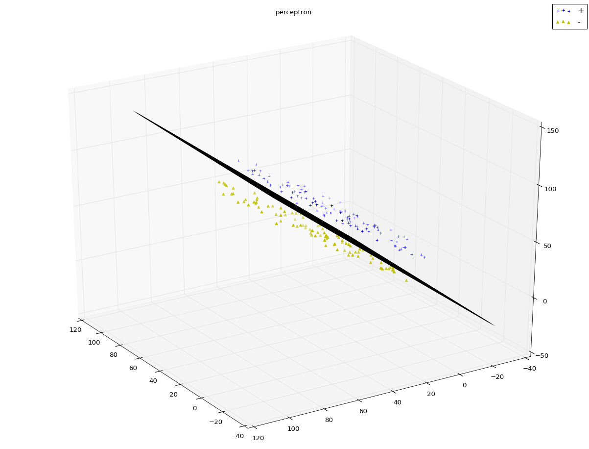
　　注：算法中，最外层循环只有在全部分类正确的这种情况下退出；内层循环从前到后遍历所有的样本点。一旦发现某个样本点是误分类点，就更新w和b，然后重新从头开始遍历所有的样本点。感知机算法的对偶形式（参考原著）其处理效果与原始算法相差不大，但是从其输出的α数组值可以看出：大多数的样本点对于最终解并没有贡献。分离超平面的位置是由少部分重要的样本点决定的。而感知机学习算法的对偶形式能够找出这些重要的样本点。这就是支持向量机的原理。

　　一开始我在create data时，公式写错了，导致所得到的数据线性不可分，此时发现算法根本无法完成迭代。可见感知机算法只能够用于线性可分数据集。　　

2、神经网络

（1）从感知机到神经网络：M-P神经元模型

　　1）每个神经元接收到来自相邻神经元传递过来的输入信号

　　2）这些输入信号通过带权重的连接进行传递

　　3）神经元接收到的总输入值将与神经元的阈值进行比较，然后通过“激活函数”处理以产生神经元输出

　　4）理论上的激活函数为阶跃函数

　　　　　　　　　　　　　　　　　　　　　　　　1,x>=0

　　　　　　　　　　　　　　　　　　　     f(x)=

　　　　　　　　　　　　　　　　　　　　　　　　0,x<0

（2）多层前馈神经网络

　　通常神经网络的结构为：1）每层神经元与下一层神经元全部互连  2）同层神经元之间不存在连接  3）跨层神经元之间也不存在连接

　　多层前馈神经网络具有以下特点：1）隐含层和输出层神经元都是拥有激活函数的功能神经元  2）输入层接收外界输入信号，不进行激活函数处理  3）最终结果由输出层神经元给出

　　神经网络的学习就是根据训练数据集来调整神经元之间的连接权重，以及每个功能神经元的阈值。

　　多层前馈神经网络的学习通常采用误差逆传播算法（error  BackPropgation，BP）：该算法是训练多层神经网络的经典算法，其从原理上就是普通的梯度下降法求最小值问题。它关键的地方在于两个：1）导数的链式法则  2）sigmoid激活函数的性质：sigmoid函数求导的结果等于自变量的乘积形式

　　多层前馈网络若包含足够多神经元的隐含层，则它就能够以任意精度逼近任意复杂度的连续函数

　　实验代码：

 from matplotlib import pyplot as plt
 from mpl_toolkits.mplot3d import Axes3D
 import numpy as np
 from sklearn.datasets import load_iris
 from sklearn.neural_network import MLPClassifier

 def creat_data_no_linear(n):
     np.random.seed(1)
     x_11=np.random.randint(0,100,(n,1))
     x_12=10+np.random.randint(-5,5,(n,1,))

     x_21 = np.random.randint(0, 100, (n, 1))
     x_22 = 20+np.random.randint(0, 10, (n, 1))

     x_31 = np.random.randint(0, 100, (int(n/10),1))
     x_32 = 20+np.random.randint(0, 10, (int(n/10), 1))

     # print(x_11)
     # print(x_12)
     # print(x_13)
     # print(x_21)
     # print(x_22)
     # print(x_23)

     # rotate 45 degrees along the X axis
     new_x_11 = x_11 * np.sqrt(2) / 2 - x_12 * np.sqrt(2) / 2
     new_x_12=x_11*np.sqrt(2)/2+x_12*np.sqrt(2)/2
     new_x_21 = x_21 * np.sqrt(2) / 2 - x_22 * np.sqrt(2) / 2
     new_x_22=x_21*np.sqrt(2)/2+x_22*np.sqrt(2)/2
     new_x_31 = x_31 * np.sqrt(2) / 2 - x_32 * np.sqrt(2) / 2
     new_x_32 = x_31 * np.sqrt(2) / 2 + x_32 * np.sqrt(2) / 2

     # print(new_x_12)
     # print(new_x_13)
     # print(new_x_22)
     # print(new_x_23)

     plus_samples=np.hstack([new_x_11,new_x_12,np.ones((n,1))])
     minus_samples=np.hstack([new_x_21,new_x_22,-np.ones((n,1))])
     err_samples=np.hstack([new_x_31,new_x_32,np.ones((int(n/10),1))])
     samples=np.vstack([plus_samples,minus_samples,err_samples])
     # print(samples)
     np.random.shuffle(samples)

     # print(plus_samples)
     # print(minus_samples)
     # print(samples)

     return  samples

 def plot_samples_2d(ax,samples):
     Y=samples[:,-1]
     # print(Y)
     position_p=Y==1 ##the position of positve class
     position_m=Y==-1 ##the position of minus class
     # print(position_p)
     # print(position_m)
     ax.scatter(samples[position_p,0],samples[position_p,1],marker='+',label="+",color='b')
     ax.scatter(samples[position_m,0],samples[position_m,1],marker='^',label='-',color='y')

 def predict_with_MLPClassifier(ax,train_data):
     train_x=train_data[:,:-1]
     train_y=train_data[:,-1]
     clf=MLPClassifier(activation='logistic',max_iter=1000)
     clf.fit(train_x,train_y)
     print(clf.score(train_x,train_y))

     x_min,x_max=train_x[:,0].min()-1,train_x[:,0].max()+2
     y_min,y_max=train_x[:,1].min()-1,train_x[:,1].max()+2
     plot_step=1

     xx,yy=np.meshgrid(np.arange(x_min,x_max,plot_step),np.arange(y_min,y_max,plot_step))
     Z=clf.predict(np.c_[xx.ravel(),yy.ravel()])
     Z=Z.reshape(xx.shape)
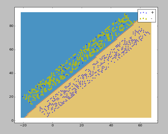
     ax.contourf(xx,yy,Z,cmap=plt.cm.Paired)

 fig=plt.figure()
 ax=fig.add_subplot(1,1,1)
 data=creat_data_no_linear(500)
 predict_with_MLPClassifier(ax,data)
 plot_samples_2d(ax,data)
 ax.legend(loc='best')
 plt.show()

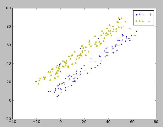
　　实验结果：

　　生成的实验数据

　　样例（对鸢尾花进行分类）代码：

 from matplotlib import pyplot as plt
 from mpl_toolkits.mplot3d import Axes3D
 import numpy as np
 from sklearn.datasets import load_iris
 from sklearn.neural_network import MLPClassifier

 def load_data():
     iris=load_iris()
     X=iris.data[:,0:2] #choose the first two features
     Y=iris.target
     data=np.hstack((X,Y.reshape(Y.size,1)))
     np.random.seed(0)
     np.random.shuffle(data)
     X=data[:,:-1]
     Y=data[:,-1]
     x_train=X[:-30]
     x_test=X[-30:]
     y_train=Y[:-30]
     y_test=Y[-30:]

     return x_train,x_test,y_train,y_test

 def neural_network_sample(*data):
     x_train,x_test,y_train,y_test=data
     cls=MLPClassifier(activation='logistic',max_iter=10000,hidden_layer_sizes=(30,))
     cls.fit(x_train,y_train)
     print("the train score:%.f"%cls.score(x_train,y_train))
     print("the test score:%.f"%cls.score(x_test,y_test))

 x_train,x_test,y_train,y_test=load_data()

 neural_network_sample(x_train,x_test,y_train,y_test)

　　实验结果：

  这里的score居然等于1。。。书上给的数据是0.8，不知道是因为算法改进了还是怎么回事。

　　注：在进行编码实现时遇到了一些小插曲，就是Anaconda的sklearn并不是完整的，当导入MLPClassifier时会出错，因为其中0.17的版本的scikit-learn中并不包括这个库。所以接下来要做的就是更新Anaconda的相关库。这时候问题就来了，更新时，网速极慢，只有6k/s，并且十几秒后就会报错，错误原因是无法连接某些网址。起初我以为是网速的问题，尝试了各种方式，调整了网络通各个端口去试都没有用，甚至想到了换网线和换网络通账号，结果还是不行。后来想到会不会是要翻墙，于是参照着这个网址：http://blog.sina.com.cn/s/blog_920b83770102xjxp.html，翻了一下，发现并不能访问youtube，这让我感到很难受。抱着试试的态度我又重新敲起了更新的指令，这次居然奇迹般的可以了！！！后来一想youtube之所以打不开，可能是浏览器的设置问题，vpn本身是可以用的。有种天道酬勤的感觉！

　　不过这也让我很好的反思了一下。遇到问题时一定要认真分析可能的原因，而不是盲目的去猜，甚至愚蠢的去多次尝试之前并没有生效的方法，这样会浪费太多的时间。解决问题一定是从可能性最大的错误着手，并且要加以分析，否则不仅时间浪费了，自信心也受到了打击，人也会弄的疲劳不堪。