CTR学习笔记&代码实现3-深度ctr模型 FNN->PNN->DeepFM

这一节我们总结FM三兄弟FNN/PNN/DeepFM，由远及近，从最初把FM得到的隐向量和权重作为神经网络输入的FNN，到把向量内/外积从预训练直接迁移到神经网络中的PNN，再到参考wide&Deep框架把人工特征交互替换成FM的DeepFM，我们终于来到了2017年。。。

以下代码针对Dense输入感觉更容易理解模型结构，针对spare输入的代码和完整代码
https://github.com/DSXiangLi/CTR

FNN

FNN算是把FM和深度学习最早的尝试之一。可以从两个角度去理解FNN：从之前Embedding+MLP的角看，FNN使用FM预训练的隐向量作为第一层可以加快模型收敛。从FM的角度来看，FM局限于二阶特征交互信息，想要学到更高阶的特征交互，在FM基础上叠加全联接层就是FNN。

补充一下Embedding直接拼接作为输入为啥收敛的这么慢，一个是参数太多一层Embedding就要N*K个参数再加上后面的全联接层，另外就是每次gradient descent只会更新和稀疏离散输入里面非0特征对应的Embedding。

模型

先看下FM的公式，FNN提取了以下的\(W,V\)来作为神经网络第一层的输入

\[\begin{align} y(x) & = w_0 + \sum_{i=1}^Nw_i x_i + \sum_{i=1}^N \sum_{j=i+1}^N <v_i,v_j> x_ix_j\\ \end{align} \]

FNN的模型结构比较简单。输入特征N维, FM隐向量维度是K

预训练FM模型提取最终的隐向量\(V = [v_1,v_2,...,v_n] \in R^{N*k} \,\, v_i \in R^{1*K}\)和权重\(w= [w_1,w2,...,w_n] w \in R^{1*N}\)
FNN模型用\(V\)和\(W\)来初始化神经网络的第一层.模型输入是由特征离散化后的one-hot矩阵拼接而成(x),每个离散特征(i)的one-hot输入都映射到它的低维embedding上\(z_i = [w_i, v_i] *x[start_i:end_i]\), 第一层是由\([z_1,z_2,...z_n]\)
两个常规的全联接层到最终给出CTR的预测。

模型结构如下

FNN几个能想到的问题有

非端到端的模型，一点都不优雅有没有
最终FNN的表现会一定程度受到预训练FM表现的限制，神经网络的最大信息量<=FM隐向量和权重所含信息量，当然这不代表FNN会比FM差因为FM对信息的提取只用了内积
从Wide&Deep角度，模型对低阶信息的提炼会比较有限
单纯的全联接层对于进一步提炼隐向量上的信息可能不够高效

代码实现

这里用了tf.contrib.framework.load_variable去读了之前FM模型的embedding和weight。感觉也可以直接把FM的variable写出来，然后FNN里用params再传进去也是可以的。

@tf_estimator_model

def model_fn(features, labels, mode, params):

    feature_columns= build_features()

    input = tf.feature_column.input_layer(features, feature_columns)

    with tf.variable_scope('init_fm_embedding'):

        # method1: load from checkpoint directly

        embeddings = tf.Variable( tf.contrib.framework.load_variable(

            './checkpoint/FM',

            'fm_interaction/v'

        ) )

        weight = tf.Variable( tf.contrib.framework.load_variable(

            './checkpoint/FM',

            'linear/w'

        ) )

        dense = tf.add(tf.matmul(input, embeddings), tf.matmul(input, weight))

        add_layer_summary('input', dense)

    with tf.variable_scope( 'Dense' ):

        for i, unit in enumerate( params['hidden_units'] ):

            dense = tf.layers.dense( dense, units=unit, activation='relu', name='dense{}'.format( i ) )

            dense = tf.layers.batch_normalization( dense, center=True, scale=True, trainable=True,

                                                   training=(mode == tf.estimator.ModeKeys.TRAIN) )

            dense = tf.layers.dropout( dense, rate=params['dropout_rate'],

                                       training=(mode == tf.estimator.ModeKeys.TRAIN) )

            add_layer_summary( dense.name, dense )

    with tf.variable_scope('output'):

        y = tf.layers.dense(dense, units= 1, name = 'output')

        tf.summary.histogram(y.name, y)

    return y

PNN

PNN的目标在paper最开始就点明了以比MLPs更有效的方式来挖掘信息。在前一篇我们就说过MLP理论上可以提炼任意信息，但也因为它太过general导致最终模型能学到模式受数据量的限制会非常有限，PNN借鉴了FM的思路来帮助MLP学到更多特征交互信息。

模型

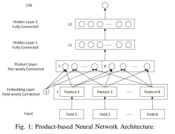
PNN给出了三种挖掘特征交互信息的方式IPNN采用向量内积，OPNN采用向量外积，concat在一起就是PNN。模型结构如下

Input层
输入是N个离散特征one-hot处理后拼接而成的高维稀疏矩阵，每个特征映射到相同维度(k)的低维embddding上
Product层
- Z是线性部分，和‘1’相乘也就是直接把N个K维Embedding拼接得到N*K的稠密矩阵copy过来
- p是特征交互部分
  - IPNN是两两特征做内积\((1*k)*(k*1)\)得到的scaler拼接成p，维度是\(O(N^2)\)
  - OPNN是两两特征做外积\((k*1)*(1*k)\)得到\(K^2\)的矩阵拼接成p，维度是\(O(K^2N^2)\)
  - PNN就是[IPNN,OPNN]

之后跟全连接层。可以发现去掉全联接层把权重都设为1，把线性部分对接到最初的离散输入那IPNN就退化成了FM。

Product层的优化

以上IPNN和OPNN的计算都有维度过高，计算复杂度过高的问题，作者进行了相应的优化。

OPNN: \(O(N^2K^2) \to O(K^2)\)
原始的OPNN，p中的每个元素都是向量外积的矩阵\(p_{i,j} \in R^{k*k}\),优化后作者对所有K*K矩阵进行了sum_pooling，也等同于先对隐向量求和\(R^{N*K} \to R^{1*K}\)再做外积\(p = \sum_{i=1}^N\sum_{j=1}^N f_if_j^T=f_{\sum}(f_{\sum})^T \, \, f_{\sum}=\sum_{i=1}^Nf_i\)
IPNN： \(O(N^2) \to O(N*K)\)
IPNN的优化又一次用到了FM的思想，内积产生的\(p \in R^{N^2}\)是对称矩阵,因此在之后全联接层的权重\(w_p\)也一定是对称矩阵。所以用矩阵分解来进行降维，假定每个神经元对应的权重\(w_p^n = \theta^n{\theta^n}^T \text{where } \theta^n \in R^N\)
\(w_p^n \odot p = \sum_{i=1}^N\sum_{j=1}^N\theta^n_i\theta^n_j<f_i,f_j>=<\sum_{i=1}^N\delta_i^n,\sum_{i=1}^N\delta_i^n>\)

PNN的几个可能可以吐槽的地方

和FNN一样对低阶特征的提炼比较有限
OPNN的部分如果不优化维度太高，在我尝试的训练集上基本是没啥用。优化后这个sum_pooling究竟还保留了什么信息，我是没太琢磨明白

代码实现

@tf_estimator_model

def model_fn(features, labels, mode, params):

    dense_feature= build_features()

    dense = tf.feature_column.input_layer(features, dense_feature) # lz linear concat of embedding

    feature_size = len( dense_feature )

    embedding_size = dense_feature[0].variable_shape.as_list()[-1]

    embedding_matrix = tf.reshape( dense, [-1, feature_size, embedding_size] )  # batch * feature_size *emb_size

    with tf.variable_scope('IPNN'):

        # use matrix multiplication to perform inner product of embedding

        inner_product = tf.matmul(embedding_matrix, tf.transpose(embedding_matrix, perm=[0,2,1])) # batch * feature_size * feature_size

        inner_product = tf.reshape(inner_product, [-1, feature_size * feature_size ])# batch * (feature_size * feature_size)

        add_layer_summary(inner_product.name, inner_product)

    with tf.variable_scope('OPNN'):

        outer_collection = []

        for i in range(feature_size):

            for j in range(i+1, feature_size):

                vi = tf.gather(embedding_matrix, indices = i, axis=1, batch_dims=0, name = 'vi') # batch * embedding_size

                vj = tf.gather(embedding_matrix, indices = j, axis=1, batch_dims= 0, name='vj') # batch * embedding_size

                outer_collection.append(tf.reshape(tf.einsum('ai,aj->aij',vi,vj), [-1, embedding_size * embedding_size])) # batch * (emb * emb)

            outer_product = tf.concat(outer_collection, axis=1)

        add_layer_summary( outer_product.name, outer_product )

    with tf.variable_scope('fc1'):

        if params['model_type'] == 'IPNN':

            dense = tf.concat([dense, inner_product], axis=1)

        elif params['model_type'] == 'OPNN':

            dense = tf.concat([dense, outer_product], axis=1)

        elif params['model_type'] == 'PNN':

            dense = tf.concat([dense, inner_product, outer_product], axis=1)

        add_layer_summary( dense.name, dense )

    with tf.variable_scope('Dense'):

        for i, unit in enumerate( params['hidden_units'] ):

            dense = tf.layers.dense( dense, units=unit, activation='relu', name='dense{}'.format( i ) )

            dense = tf.layers.batch_normalization( dense, center=True, scale=True, trainable=True,

                                                   training=(mode == tf.estimator.ModeKeys.TRAIN) )

            dense = tf.layers.dropout( dense, rate=params['dropout_rate'],

                                       training=(mode == tf.estimator.ModeKeys.TRAIN) )

            add_layer_summary( dense.name, dense)

    with tf.variable_scope('output'):

        y = tf.layers.dense(dense, units=1, name = 'output')

        add_layer_summary( 'output', y )

    return y

DeepFM

DeepFM是对Wide&Deep的Wide侧进行了改进。之前的Wide是一个LR，输入是离散特征和交互特征，交互特征会依赖人工特征工程来做cross。DeepFM则是用FM来代替了交互特征的部分，和Wide&Deep相比不再依赖特征工程，同时cross-column的剔除可以降低输入的维度。

和PNN/FNN相比，DeepFM能更多提取到到低阶特征。而且上述这些模型间直接并不互斥，比如把DeepFM的FMLayer共享到Deep部分其实就是IPNN。

模型

Wide部分就是一个FM，输入是N个one-hot的离散特征，每个离散特征对应到等长的低维(k)embedding上，最终输出的就是之前FM模型的output。并且因为这里不需要像IPNN一样输出隐向量，因此可以使用FM降低复杂度的trick。

Deep部分和Wide部分共享N*K的Embedding输入层，然后跟两个全联接层

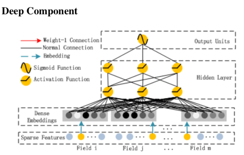
Deep和Wide联合训练，模型最终的输出是FM部分和Deep部分权重为1的简单加和。联合训练共享Embedding也保证了二阶特征交互学到的Embedding会和高阶信息学到的Embedding的一致性。

代码实现

@tf_estimator_model

def model_fn(features, labels, mode, params):

    dense_feature, sparse_feature = build_features()

    dense = tf.feature_column.input_layer(features, dense_feature)

    sparse = tf.feature_column.input_layer(features, sparse_feature)

    with tf.variable_scope('FM_component'):

        with tf.variable_scope( 'Linear' ):

            linear_output = tf.layers.dense(sparse, units=1)

            add_layer_summary( 'linear_output', linear_output )

        with tf.variable_scope('second_order'):

            # reshape (batch_size, n_feature * emb_size) -> (batch_size, n_feature, emb_size)

            emb_size = dense_feature[0].variable_shape.as_list()[0] # all feature has same emb dimension

            embedding_matrix = tf.reshape(dense, (-1, len(dense_feature), emb_size))

            add_layer_summary( 'embedding_matrix', embedding_matrix )

            # Compared to FM embedding here is flatten(x * v) not v

            sum_square = tf.pow( tf.reduce_sum( embedding_matrix, axis=1 ), 2 )

            square_sum = tf.reduce_sum( tf.pow(embedding_matrix,2), axis=1 )

            fm_output = tf.reduce_sum(tf.subtract( sum_square, square_sum) * 0.5, axis=1, keepdims=True)

            add_layer_summary('fm_output', fm_output)

    with tf.variable_scope('Deep_component'):

        for i, unit in enumerate(params['hidden_units']):

            dense = tf.layers.dense(dense, units = unit, activation ='relu', name = 'dense{}'.format(i))

            dense = tf.layers.batch_normalization(dense, center=True, scale = True, trainable=True,

                                                  training=(mode ==tf.estimator.ModeKeys.TRAIN))

            dense = tf.layers.dropout( dense, rate=params['dropout_rate'], training = (mode==tf.estimator.ModeKeys.TRAIN))

            add_layer_summary( dense.name, dense )

    with tf.variable_scope('output'):

        y = dense + fm_output + linear_output

        add_layer_summary( 'output', y )

    return y

CTR学习笔记&代码实现系列

https://github.com/DSXiangLi/CTR

CTR学习笔记&代码实现1-深度学习的前奏LR->FFM
CTR学习笔记&代码实现2-深度ctr模型 MLP->Wide&Deep

资料

Huifeng Guo et all. "DeepFM: A Factorization-Machine based Neural Network for CTR Prediction," In IJCAI,2017.
Qu Y, Cai H, Ren K, et al. Product-based neural networks for user response prediction,2016 IEEE
Weinan Zhang, Tianming Du, and Jun Wang. Deep learning over multi-field categorical data - - A case study on user response
https://daiwk.github.io/posts/dl-dl-ctr-models.html
https://zhuanlan.zhihu.com/p/86181485