Tree - Decision Tree with sklearn source code

After talking about Information theory, now let's come to one of its application - Decision Tree! Nowadays, in terms of prediction power, there are many ensemble methods based on tree that can beat Decision Tree generally. However I found it necessary to talk about Decision Tree before we talk about other advanced methods mainly for 2 reasons:

Decision Tree is often used as the base learner for many ensemble methods, like GBM (GBRT), AdaBoost, xgBoost and etc.
Decision Tree is very straightforward, and is outstanding in its explanatory power. It is freuently used in model interpretation, like DT-surrogate.

In this post, I will go through how to build decision tree for both classification and regression problem along with some discussion over several issues. As the topics says, the structure of this post will mimic the way the Decision Tree Class is defined in sklearn. Since sklearn is built upon CART, we will mainly talk about CART. In the end we will have a comparison between CART and other Tree Building algorithm.

Decision Tree Builder

Ideally for a perfect tree, the tree leaf should have only 1 class for classification problem and should be constant for regression problem. Although perfect situation cannot be met, but training process should serve this purpose.

Basically each split should increase the purity of the sample in the node - more sample from same class (classification) or more clustered target value (regression).

Let's first define the problem:

For N sample, $(x_i,y_i), i \in [1,2,...N]$, where x is a P-dimension vector.

Tree splits the sample in to M region, $R_1... R_M$

Each sample will have following prediction.

\[f(x) = \sum_i^M{c_m I(x \in R_m)}
\]

For regression, $c_m$ will the be average of all samples in that leaf, if the loss metric is sum of squares. For classification, $c_m$ will be the majority class in that leaf.

1. Criterion - theory

Now we know the target of the problem, how are we going to bulid the tree?

For classification problem, when target value has K classes, at leaf m, probability of the majority class will be :

\[{\hat{p}}_{mk} =\frac{1}{N_m} \sum_{x_i \in R_m}{ I(y_i=k)}
\]

For each split, we want to maximize reduction in impurity, or in other words the minimum impurity for sample in current node. Do you still recall in the previous post we talk about cross-entropy and Information gain, where

\[IG = H(Y) - H(Y|X)
\]

\[H(Y) =-\sum_{k=1}^{K}{p_k \log{p_k}}
\]

Bingo! Cross-entropy is usually used as a splitting criterion. Information gain is exactly the impurity reduction after the split. So for cross-entropy criterion, we want the largest information gain for each split to achieve minimum conditional cross-entropy after the split. So we iterate across all the variables and their value to find the optimal split (variable j and split point s), which minimize the weighted sum of cross-entropy of left node and right node.

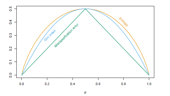
\[\min_{j,s}-[\frac{N_L}{N_m}\sum_{k=1}^{K}{\hat{p}_{Lk} \log{\hat{p}_{Lk}}} +\frac{N_R}{N_m}\sum_{k=1}^{K}{\hat{p}_{Rk} \log{\hat{p}_{Rk}}} ]
\]

Besides cross-entropy, we also have misclassification rate and Gini Index. Let's compare how they calculate impurity of each node:

Misclassification Rate : $ \frac{1}{N_m}\sum_{x_i \in R_m}{ I(y_i \neq k)} = 1- {\hat{p}}_{mk} $

Gini Index : $\sum_{k=1}^{K}{\hat{p}_{mk}(1-\hat{p}_{mk})}$

Cross-entropy : $-\sum_{k=1}^{K}{\hat{p}_{mk}\log(\hat{p}_{mk})}$

For a 2-class classification, the above 3 metric has the following distribution over p. (Entropy is scaled to pass(0.5,0.5))

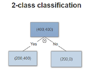
From above distribution, we can tell that Gini and entropy are more sensitive to the pure node, where p close to 0 or 1. For example a 2 class classification tree

Metric	Split 1	Split 2
Split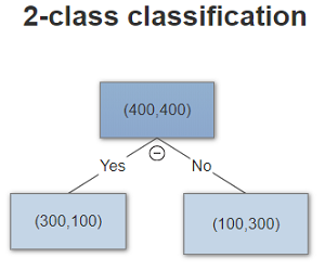
Missclassification rate	0.25	0.25
Gini	3/16	1/6
Cross-entropy	0.81	0.69

where we can see Gini and Cross-entropy has smaller impurity for split 2.

In summary

Misclassifiaction Rate is not diffferentiable. Therefore in sklearn Tree model, only Gini and cross-entropy are used.
Gini and Cross-entropy have no significant different. But cross-entropy can be slower due to the log computation.
Gini and Cross-entropy have preference for pure node, see above example.

Issue1: Instability

Tree model is very sensitive to the change in data. A small change in the input can lead to an entire different tree. Partly because tree is built in a greedy way, instead of search for global optimum. Also because decision tree make hard split at each node. If a sample goes to the wrong node at first, then this error will be carried all the way to the leaf.

For regression problem, we only need to change the above criterion. If we use mean square error, then at each split we search for optimal split (variable j and split point s) by minimizing:

\[\min_{j,s}[ \min_{c_1} \sum_{x_i \in R_L}{ (y_i - c_1)^2 } + \min_{c_2} \sum_{x_i \in R_R}{ (y_i - c_2)^2 }]
\]

where $R_L$$R_R$ is the left and right node, and $c_1$$c_2$ is the average of sample in the node.

Issue2: Binary Split

Decision is default to binary split. Because multi-split reduce the number of sample in the node too fast. Since we can visit each variable more than 1 time, we can achieve multi-split by doing multiple binary split on same variable. However when input are huge, even binary split may reduce the sample too fast.

Issue3: Lack of smoothness

For regression problem, the prediction is the average of samples in the final leaf. Although setting the minimal number of sample in the leaf can help over fitting, it may make the prediction between samples not continuous.

2. Criterion - sklearn source code

In sklearn, following criterion class for regression and classification are defined. Criterion Class calculates the impurity of node and the reduction of impurity after split. I extract the source code related to the criterion calculation.

CRITERIA_CLF = {"gini": _criterion.Gini, "entropy": _criterion.Entropy}

CRITERIA_REG = {"mse": _criterion.MSE, "friedman_mse": _criterion.FriedmanMSE, "mae": _criterion.MAE}

Gini

for k in range(self.n_outputs):

    sq_count = 0.0

    for c in range(n_classes[k]):

        count_k = sum_total[c]

        sq_count += count_k * count_k

    gini += 1.0 - sq_count / (self.weighted_n_node_samples *

                              self.weighted_n_node_samples)

Entropy

for k in range(self.n_outputs):

    for c in range(n_classes[k]):

        count_k = sum_total[c]

        if count_k > 0.0:

            count_k /= self.weighted_n_node_samples

            entropy -= count_k * log(count_k)

MSE

In order to compute MSE in O(#sample), it decompose $\sum(y_i - \hat{y})^2$ into $\sum{y_i^2} - n\hat{y}^2$

#self.sq_sum_total is the weighted sum of y^2

#sum_total is the weighted sum of y

impurity = self.sq_sum_total / self.weighted_n_node_samples

for k in range(self.n_outputs):

    impurity -= (sum_total[k] / self.weighted_n_node_samples)**2.0

MAE

When using mean absolute error as criterion, instead of taking average, we should take median of all samples in the leaf as prediction.

for k in range(self.n_outputs):

    for p in range(self.start, self.end):

        i = samples[p]

        y_ik = y[i * self.y_stride + k]

        impurity += <double> fabs((<double> y_ik) - <double> self.node_medians[k])

FriedmanMSE

This criterion is built upon MSE, which defines a new way to calculate impurity reduction. It maximize the difference between the mean of left node and right node, in other words best split should make the left and right node more distinguishable.

diff = (self.weighted_n_right * total_sum_left -

        self.weighted_n_left * total_sum_right) / self.n_outputs

diff * diff / (self.weighted_n_left * self.weighted_n_right *

                       self.weighted_n_node_samples)

3. Splitter - sklearn source code

After talking about how to evaluate each split, we come to splitter itself. Of course the traditional way of Decision Tree learning process is to choose the best split in a greedy way. So at each split we search across all variable and all the value of this variable to find the best split.

Additionally sklearn also support 'Random Split'. Instead of searching for the best split, it searches for random best split, where random features are drew, random value are evaluated and we use the best split from these random splits.

Definitely random split is not as good as best split independently. However this method has its own advantage in smaller computation time and less prone to over-fitting.

Also Random Splitter is frequently used in Bagging and Boosting method, like random forest. We will go back to this in following post.

Decision Tree Stopping and pruning

Now we know how to build the tree from top to the bottom, there is another problem to solve - when shall we stop?

The biggest challenge of tree model is over fitting. Under the extreme situation, where each leaf has only one sample, we can always achieve 0 error for training. But the model will not perform good on unseen data set, because it learns too many features unique to the training set, instead of the general distribution.

Now let's see how sklearn deal with over fitting in their Decision Tree class. Following hyper parameters are used:

Parameter	Description
min_samples_split	Minimum number of samples in an internal node.
min_samples_leaf	Minimum number of samples in a leaf. Setting this value too small can easily lead to over fitting. The extreme condition is 1 sample per leaf.
min_weight_leaf	Minimum weight in a leaf. Only used when the sample is not equally weighted
max_depth	Maximal tree depth. A key parameter to your model, especially when input features are very big.
min_impurity_split	When impurity < threshold then stop growing.
min_impurity_decrease	If impurity decrease < threshold then stop growing. However it is possible that impurity decrease relies on interation of 2 variable. see example belows
max_leaf_nodes	Maximal number of leafs. when this parameter is not null Best-First search, otherwise Depth-First search is used.

In sklearn, above parameter are used together in following way for early stopping.

is_leaf = (depth > self.max_depth or

           n_node_samples < self.min_samples_split or

           n_node_samples < 2 * self.min_samples_leaf or

           weighted_n_node_samples < 2 * self.min_weight_leaf or

           impurity <= min_impurity_split)

if not is_leaf:

    splitter.node_split(impurity, &split, &n_constant_features)

    ##splitter calculate the impurity before and after split.

    is_leaf = (is_leaf or split.pos >= end or

               split.improvement + EPSILON < min_impurity_decrease)

Util now it seems like that we only talk about early stopping. That's is because currently sklearn doesn't support post-pruning yet.

But why we need pruning anyway? The major problem comes from one hyper-parameter - min_impurity_decrease. Andrew Moore gives a very good example for this:

y = a xor b. And the training sample is following:

a	b	y
0	0	0
0	1	1
1	0	0
1	1	0

Here IG = 0 no matter we split on a or b. However if we split on both a and b, we can perfectly fit the sample. The idea here is because of the interaction between input features, calculating impurity decrease only on current node can be short-sighted.

One way to overcome above problem is to grow a very large tree and prune the leaf from bottom to the top, where most of the useful interactions are already considered. Take regression tree as an example:

We define $T \subset T_0$ as a sub tree, which reaches an optimal balance between the number of nodes and accuracy as following:

\[C_a(T) = \sum_{m=1}^{|T|} N_mQ_m(T) + \alpha |T|
\]

where $N_m =\# \{x_i \in R_m\}$ is the number of sample in leaf m. $Q_m(T)$ is the mean error of leaf m, and $|T|$ is the total number of nodes in the tree.

To find the minimum of $C_a(T)$, we do a greedy search from the bottom to the top called weakest link pruning. We successively removed the node with the minimal increase in error till root, among which we find the best sub tree. Of course here $\alpha$ is a hyper parameter too. The higher it is, the smaller tree we will get. And we can tune this variable through cross-validation.

Other useful details

1. Missing value handling

Missing value has always been a headache to data analyst. And it is also a crucial advantage of tree algorithm in some of its implementation. Usually there are a few ways to handle missing value:

Remove records with missing value
Imputation, replace missing value to sample mean, median or other stats. The key here is to have minimal impact on the original distribution. Here is a example of how to use Imputer to fill in missing value
Create additional category. This is unique to tree method, where missing value can be considered as a separate class. Sometimes missing value itself indeed contain information. Under this situation imputation will lose information.
Surrogate. This is another fancy way of dealing with missing value. where we use correlated variable to substitute missing value. I will talk about this in detail later in the Model Interpretation post.

You need to be very careful when dealing with missing value in different library. Different libraries treat missing value differently. Small problem is you may see your validation score being nan. Bigger problem is an additional category is created by default and you don't even know that. So I suggest you process the missing value before training.

Advantage: Immune to multicolinearity

Above surrogate is a good evidence that tree can handle multicolinearity. Because if 2 features are highly correlated then after the one with higher IG is used, the other feature becomes less likely to be picked.

2. Max_feature

This parameter can also help over fitting problem. At each split we only consider part of the feature. Similar to Random Split and also the dropout method in neural network, we want the weight on different features to be more spread out. This feature is more useful in the boosting/bagging method. So we will come back to it later.

Different Model Comparison

Besides CART, there are many other tree (tree like) algorithms, where the major difference comes from: criterion(loss metric), splitter. Here we will talk about ID3, C4.5, MARS, and PRIM, mainly because they are related to a few issues we mentioned above.

Method	Target	Input	Criterion	Splitter
ID3	classification	categorical	Information Gain	multi-split
C4.5	classification	Both	Information Gain Ratio	multi-split
MARS	regression	numeric	MSE	binary-split
PRIM	regression	Both	Max target mean	Box peeling

ID3

ID3 is the earliest version of Tree building algo. And as we mentioned above, its multi-split splitter is prone to over fitting. It doesn't have missing value handling, and only take in categorical input for classification problem.
C4.5

C4.5 improves upon ID3. It adds missing value handling, and treat categorical with numeric encoding. And the most important part is its implement of Information Gain Ratio.

As we mentioned above, IG and GINI has preference over pure node. And this problem is amplified given C4.5 do multi-split not binary split. If we have high-dimension categorical input, then it can over fit easily by splitting on such input. IGR is designed to solve this:

\[IGR = \frac{H(Y) - H(Y|X)}{H(X)} = \frac{IG}{H(X)}
\]

If the splitting variable has many values, then itself will have higher entropy and penalize its information gain.

PRIM (Patient Rule Induction Method)

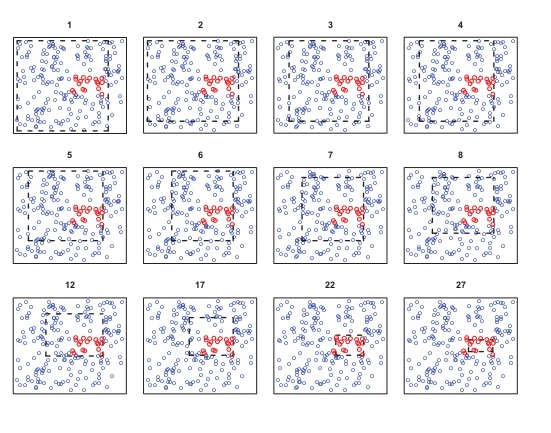
Instead of doing binary split on each variable, PRIM partition the features into box ($a<x_1<b$, $c<x_2<d$), like below:

Each iteration it peels one side of the box by $\alpha$ to maximize the average of target value in the box.

PRIM further solves one issue we mentioned above - Binary tree split. Because peeling method shrinks sample in the box slower than binary split. The shrinking speed is $O(log(N)/log(1-a))$ vs. $O(log(N)/log(2))$
MARS - Multivariate Adaptive regression.

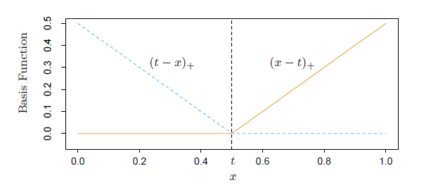
The invention of MARS is the linear basis function, which is also know as rectifier function (RELU) in neural network.

\[(x-t)_+ = max(x-t,0)
\]

MARS has a collection of basis function ,where for each variable we have a pair of linear basis function, see below:

In each iteration, we search for the best pair of basis function (variable, t) that leads to largest decrease in training error. And the new pair of basis function can interact with the current term in following ways:

1.multiply by existing intercept.

2.multiply by existing basis function.

For example

\[Y = (x_1 -1)_+ + (x_1 -1)_+ \cdot (x_2 -8)_+
\]

And if you consider each split in CART as an indicator function: I(x-a>0) and replace basis function with indicator, then MARS becomes regression tree. In other words MARS can be viewed as a locally weighted regression, regression tree is a locally weighted constant (sample mean in each leaf). That's why MARS can solve Issue3 of tree - lack of smoothness.

In the following we will talk about all kinds of ensemble method.

To be continued.

Reference

1 Friedman, J.H (1991) Multivariate adaptive regression splines.

2 scikit-learn tutorial http://scikit-learn.org/stable/modules/classes.html#module-sklearn.tree

3 T. Hastie, R. Tibshirani and J. Friedman. “Elements of Statistical Learning”, Springer, 2009.

4 L. Breiman, J. Friedman, R. Olshen, and C. Stone, “Classification and Regression Trees”, Wadsworth, Belmont, CA, 1984.

5 Andrew Moore Tutorial http://www.cs.cmu.edu/~./awm/tutorials/dtree.html