CSharpGL(54)用基于图像的光照(IBL)来计算PBR的Specular部分
CSharpGL(54)用基于图像的光照(IBL)来计算PBR的Specular部分
接下来本系列将通过翻译(https://learnopengl.com)这个网站上关于PBR的内容来学习PBR(Physically Based Rendering)。
本文对应(https://learnopengl.com/PBR/IBL/Specular-IBL)。
原文虽然写得挺好,但是仍旧不够人性化。过一阵我自己总结总结PBR,写一篇更容易理解的。
正文
In the previous tutorial we've set up PBR in combination with image based lighting by pre-computing an irradiance map as the lighting's indirect diffuse portion. In this tutorial we'll focus on the specular part of the reflectance equation:
在上一篇教程中我们已经用IBL(基于图像的光照)来解决了PBR的一个问题:用预计算的辐照度贴图作为非直接光照的diffuse部分。在本教程中我们将关注反射率方程中的speclar部分。

You'll notice that the Cook-Torrance specular portion (multiplied by kS) isn't constant over the integral and is dependent on the incoming light direction, but also the incoming view direction. Trying to solve the integral for all incoming light directions including all possible view directions is a combinatorial overload and way too expensive to calculate on a real-time basis. Epic Games proposed a solution where they were able to pre-convolute the specular part for real time purposes, given a few compromises, known as the split sum approximation.
你会注意到Cook-Torrance的specular部分(乘以kS的那个)在积分上不是常量,它既依赖入射光方向,又依赖观察者方向。对所有入射光反向和所有观察者方向的乘积的积分进行求解,是过载又过载,对于实时计算是太过昂贵了。Epic游戏公司提出了一个解决方案(被称为拆分求和近似),用一点妥协,通过预计算卷积实现了specular部分的实时计算。
The split sum approximation splits the specular part of the reflectance equation into two separate parts that we can individually convolute and later combine in the PBR shader for specular indirect image based lighting. Similar to how we pre-convoluted the irradiance map, the split sum approximation requires an HDR environment map as its convolution input. To understand the split sum approximation we'll again look at the reflectance equation, but this time only focus on the specular part (we've extracted the diffuse part in the previous tutorial):
拆分求和近似方案,将反射率方程的specular部分拆分为两个单独的部分,我们可以分别对齐进行卷积,之后再结合起来。在shader中可以实现这样的specular的IBL。与我们预计算辐照度贴图相似,拆分求和近似方案需要一个HDR环境贴图作为输入。为了理解这个方案,我们再看一下反射率方程,但这次只关注specular部分(我们已经在上一篇教程中分离出了diffuse部分):

For the same (performance) reasons as the irradiance convolution, we can't solve the specular part of the integral in real time and expect a reasonable performance. So preferably we'd pre-compute this integral to get something like a specular IBL map, sample this map with the fragment's normal and be done with it. However, this is where it gets a bit tricky. We were able to pre-compute the irradiance map as the integral only depended on ωi and we could move the constant diffuse albedo terms out of the integral. This time, the integral depends on more than just ωi as evident from the BRDF:
由于和辐照度卷积相同的原因(性能),我们不能实时求解specular部分的积分,还期待一个可接受的性能。所以我们倾向于预计算这个积分,得到某种specular的IBL贴图,用片段的法线在贴图上采样,得到所需结果。但是,这里比较困难。我们能预计算辐照度贴图,是因为它的积分只依赖ωi,而且我们还能吧diffuse颜色项移到积分外面。这次,从BRDF公式上可见,积分不止依赖一个ωi。

This time the integral also depends on wo and we can't really sample a pre-computed cubemap with two direction vectors. The position p is irrelevant here as described in the previous tutorial. Pre-computing this integral for every possible combination of ωi and ωo isn't practical in a real-time setting.
这次,积分还依赖于wo,我们无法对有2个方向向量的预计算cubemap贴图进行采样。这里的位置p是无关的,我们在上一篇教程中讲过。在实时系统中预计算这个积分的ωi和ωo的每种组合,是不实际的。
Epic Games' split sum approximation solves the issue by splitting the pre-computation into 2 individual parts that we can later combine to get the resulting pre-computed result we're after. The split sum approximation splits the specular integral into two separate integrals:
Epic游戏公司的拆分求和近似方案解决了这个问题:把预计算拆分为2个互相独立的部分,且之后可以联合起来得到我们需要的预计算结果。拆分求和近似方案将specular积分拆分为2个独立的积分:

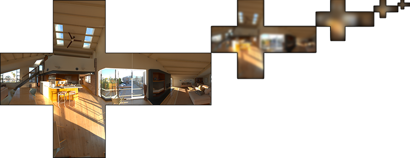
The first part (when convoluted) is known as the pre-filtered environment map which is (similar to the irradiance map) a pre-computed environment convolution map, but this time taking roughness into account. For increasing roughness levels, the environment map is convoluted with more scattered sample vectors, creating more blurry reflections. For each roughness level we convolute, we store the sequentially blurrier results in the pre-filtered map's mipmap levels. For instance, a pre-filtered environment map storing the pre-convoluted result of 5 different roughness values in its 5 mipmap levels looks as follows:
卷积时的第一部分被称为pre-filter环境贴图(类似辐照度贴图),是个预计算的环境卷积贴图,但这次它考虑了粗糙度。对于增长的粗糙度level,环境贴图用更散射的采样向量进行卷积,这造成了更模糊的反射。对我们卷积的每个粗糙度level,我们依次在pre-filter贴图的mipmap层上保存它。例如,一个保存着预计算结果的5个不同粗糙度(用6个mipmap层)的pre-fitler环境贴图如下图所示:
We generate the sample vectors and their scattering strength using the normal distribution function (NDF) of the Cook-Torrance BRDF that takes as input both a normal and view direction. As we don't know beforehand the view direction when convoluting the environment map, Epic Games makes a further approximation by assuming the view direction (and thus the specular reflection direction) is always equal to the output sample direction ωo. This translates itself to the following code:
Cook-Torrance函数以法线和观察者方向为输入,我们用这个函数生成采样的方向向量和散射强度。卷积环境贴图时,我们无法提前预知观察者方向,Epic游戏公司又做了个近似,假设观察者方向(即specular反射方向)总是等于输出采样方向ωo。相应的代码如下:
 vec3 N = normalize(w_o);

 vec3 R = N;

 vec3 V = R;
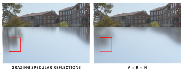
This way the pre-filtered environment convolution doesn't need to be aware of the view direction. This does mean we don't get nice grazing specular reflections when looking at specular surface reflections from an angle as seen in the image below (courtesy of the Moving Frostbite to PBR article); this is however generally considered a decent compromise:
这样,pre-filter环境贴图就不需要知道观察者方向。这意味着,在从下图(感谢Moving Frostbite to PBR 文章)所示的角度观察光滑表面反射时,我们得不到比较好的掠角反射结果。但是这一般被认为是相当好的折衷方案了。
The second part of the equation equals the BRDF part of the specular integral. If we pretend the incoming radiance is completely white for every direction (thus L(p,x)=1.0) we can pre-calculate the BRDF's response given an input roughness and an input angle between the normal n and light direction ωi, or n⋅ωi. Epic Games stores the pre-computed BRDF's response to each normal and light direction combination on varying roughness values in a 2D lookup texture (LUT) known as the BRDF integration map. The 2D lookup texture outputs a scale (red) and a bias value (green) to the surface's Fresnel response giving us the second part of the split specular integral:
方程的第二部分是specular积分的BRDF部分。如果我们假设入射光在所有方向上都是白色(即L(p,x)=1.0),我们就能预计算BRDF对给定粗糙度和入射角(法线n和入射方向ωi的夹角,或n⋅ωi)的返回值。Epic游戏公司保存了预计算的BRDF对每个法线+入射方向组合的返回值,保存到一个二维查询纹理(LUT)上,即BRDF积分贴图。这个二维查询纹理输出的是表面的菲涅耳效应的一个缩放和偏移值,也就是拆分开的specular积分的第二部分。
(我不懂这是啥)
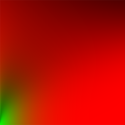
We generate the lookup texture by treating the horizontal texture coordinate (ranged between 0.0 and 1.0) of a plane as the BRDF's input n⋅ωi and its vertical texture coordinate as the input roughness value. With this BRDF integration map and the pre-filtered environment map we can combine both to get the result of the specular integral:
我们将纹理坐标的U(从0.0到1.0)作为BRDF的n⋅ωi参数,将V坐标视为粗糙度参数,以此生成查询纹理。现在我们就可以联合BRDF积分贴图和pre-filter环境贴图来得到specular的积分结果:
 float lod = getMipLevelFromRoughness(roughness);

 vec3 prefilteredColor = textureCubeLod(PrefilteredEnvMap, refVec, lod);

 vec2 envBRDF = texture2D(BRDFIntegrationMap, vec2(NdotV, roughness)).xy;

 vec3 indirectSpecular = prefilteredColor * (F * envBRDF.x + envBRDF.y)
This should give you a bit of an overview on how Epic Games' split sum approximation roughly approaches the indirect specular part of the reflectance equation. Let's now try and build the pre-convoluted parts ourselves.
这些应该让你大体上理解,Epic游戏公司的拆分求和近似方案是如何计算反射率方程的非直接specular部分的。现在我们试试自己构建预卷积部分。
预卷积HDR环境贴图
Pre-filtering an environment map is quite similar to how we convoluted an irradiance map. The difference being that we now account for roughness and store sequentially rougher reflections in the pre-filtered map's mip levels.
预卷积一个环境贴图,与我们卷积辐照度贴图类似。不同点在于,我们现在要考虑粗糙度,并且将越来越粗糙的反射情况依次保存到贴图的各个mipmap层里。
First, we need to generate a new cubemap to hold the pre-filtered environment map data. To make sure we allocate enough memory for its mip levels we call glGenerateMipmap as an easy way to allocate the required amount of memory.
首先,我们需要生成一个cubemap对象,用于保存pre-filter的环境贴图数据。为保证我们为它的mipmap层分配了足够的内存,我们使用glGenerateMipmap这一简便方式来分配需要的内存。
 unsigned int prefilterMap;

 glGenTextures(, &prefilterMap);

 glBindTexture(GL_TEXTURE_CUBE_MAP, prefilterMap);

 for (unsigned int i = ; i < ; ++i)

 {

     glTexImage2D(GL_TEXTURE_CUBE_MAP_POSITIVE_X + i, , GL_RGB16F, , , , GL_RGB, GL_FLOAT, nullptr);

 }

 glTexParameteri(GL_TEXTURE_CUBE_MAP, GL_TEXTURE_WRAP_S, GL_CLAMP_TO_EDGE);

 glTexParameteri(GL_TEXTURE_CUBE_MAP, GL_TEXTURE_WRAP_T, GL_CLAMP_TO_EDGE);

 glTexParameteri(GL_TEXTURE_CUBE_MAP, GL_TEXTURE_WRAP_R, GL_CLAMP_TO_EDGE);

 glTexParameteri(GL_TEXTURE_CUBE_MAP, GL_TEXTURE_MIN_FILTER, GL_LINEAR_MIPMAP_LINEAR);

 glTexParameteri(GL_TEXTURE_CUBE_MAP, GL_TEXTURE_MAG_FILTER, GL_LINEAR);

 glGenerateMipmap(GL_TEXTURE_CUBE_MAP);
Note that because we plan to sample the prefilterMap its mipmaps you'll need to make sure its minification filter is set to GL_LINEAR_MIPMAP_LINEAR to enable trilinear filtering. We store the pre-filtered specular reflections in a per-face resolution of 128 by 128 at its base mip level. This is likely to be enough for most reflections, but if you have a large number of smooth materials (think of car reflections) you may want to increase the resolution.
注意,因为我们计划对prefilterMap 的各层mipmap采样,你需要确保它的最小过滤参数设置为GL_LINEAR_MIPMAP_LINEAR ,这样才能启用三线过滤。以128x128像素为mipmap基层(第一层),我们将pre-filter的反射情况保存到cubemap的各个面上。这对大多数反射情况都足够用,但是如果你有大量光滑材质(例如汽车的反射),你可能需要增加分辨率。
In the previous tutorial we convoluted the environment map by generating sample vectors uniformly spread over the hemisphere Ω using spherical coordinates. While this works just fine for irradiance, for specular reflections it's less efficient. When it comes to specular reflections, based on the roughness of a surface, the light reflects closely or roughly around a reflection vector r over a normal n, but (unless the surface is extremely rough) around the reflection vector nonetheless:
在之前的教程中,我们用球坐标均匀地在半球上进行采样,实现了对环境贴图的卷积。虽然这对辐照度贴图很好用,但是对specular反射就不够高效。谈到specular反射时,根据表面粗糙度的不同,the light reflects closely or roughly around a reflection vector r over a normal n, but (unless the surface is extremely rough) around the reflection vector nonetheless:

The general shape of possible outgoing light reflections is known as the specular lobe. As roughness increases, the specular lobe's size increases; and the shape of the specular lobe changes on varying incoming light directions. The shape of the specular lobe is thus highly dependent on the material.
光反射的可能形状被称为specular叶。随着粗糙度增加,specular叶的尺寸也增加,它的形状随入射光方向而变化。因此它的形状高度依赖材质。
When it comes to the microsurface model, we can imagine the specular lobe as the reflection orientation about the microfacet halfway vectors given some incoming light direction. Seeing as most light rays end up in a specular lobe reflected around the microfacet halfway vectors it makes sense to generate the sample vectors in a similar fashion as most would otherwise be wasted. This process is known as importance sampling.
对于微平面模型,我们可以将specular叶想象为,对给定的入射光方向,微平面半向量的朝向。鉴于大多数光线都在specular叶范围内,就可以合理地用这种方式生成采样向量(反正其他被浪费的都是少数)。这个过程被称为重要性采样
蒙特卡罗积分和重要性采样
To fully get a grasp of importance sampling it's relevant we first delve into the mathematical construct known as Monte Carlo integration. Monte Carlo integration revolves mostly around a combination of statistics and probability theory. Monte Carlo helps us in discretely solving the problem of figuring out some statistic or value of a population without having to take all of the population into consideration.
为真正理解自行车采样,我们要先研究一些“蒙特卡罗积分”的数学概念。蒙特卡罗积分围绕统计学和概率理论,帮助我们用离散的方式解决统计或求值问题,且不需要考虑所有的样本。
For instance, let's say you want to count the average height of all citizens of a country. To get your result, you could measure every citizen and average their height which will give you the exact answer you're looking for. However, since most countries have a considerable population this isn't a realistic approach: it would take too much effort and time.
例如,假设你想统计一个国家的所有国民的平均身高。为得到这个结果,你可以测量每个人,然后得到准确的答案。但是,显示这不可能实现,它太费时间和精力了。
A different approach is to pick a much smaller completely random (unbiased) subset of this population, measure their height and average the result. This population could be as small as a 100 people. While not as accurate as the exact answer, you'll get an answer that is relatively close to the ground truth. This is known as the law of large numbers. The idea is that if you measure a smaller set of size N of truly random samples from the total population, the result will be relatively close to the true answer and gets closer as the number of samples N increases.
另一个办法是,挑选一个完全随机的人口子集,测量他们的身高,求平均值。这个子集可能小到100人。虽然不是准确答案,但是相对来说也很接近。这就是“大数定律”。其思想是,如果你测量完整数据的一个完全随机的子集(数量为N),那么结果会相对接近真实答案,且随着N的增加,会更接近。
Monte Carlo integration builds on this law of large numbers and takes the same approach in solving an integral. Rather than solving an integral for all possible (theoretically infinite) sample values x, simply generate N sample values randomly picked from the total population and average. As N increases we're guaranteed to get a result closer to the exact answer of the integral:
蒙特卡罗积分基于这个“大数定律”,用它来解决积分问题。与其计算所有可能的(理论上无限的)采样值x,不如简单地随机生成N个采样值,然后求平均值。随着N增加,我们就能保证得到一个越来越接近真实答案的积分结果:

To solve the integral, we take N random samples over the population a to b, add them together and divide by the total number of samples to average them. The pdf stands for the probability density function that tells us the probability a specific sample occurs over the total sample set. For instance, the pdf of the height of a population would look a bit like this:
为求解此积分,我们在a到b之间采集N个随机值,加起来,求平均值。那个pdf代表概率密度函数,它告诉我们一个特定采样值在整个样品集中出现的概率。例如,高度的pdf如下图所示:

From this graph we can see that if we take any random sample of the population, there is a higher chance of picking a sample of someone of height 1.70, compared to the lower probability of the sample being of height 1.50.
从此图中我们可以看到,如果我们随机采集一个样品,采到1.70的概率比其他(如1.50)的概率更高。
When it comes to Monte Carlo integration, some samples might have a higher probability of being generated than others. This is why for any general Monte Carlo estimation we divide or multiply the sampled value by the sample probability according to a pdf. So far, in each of our cases of estimating an integral, the samples we've generated were uniform, having the exact same chance of being generated. Our estimations so far were unbiased, meaning that given an ever-increasing amount of samples we will eventually converge to the exact solution of the integral.
对于蒙特卡罗积分,有的采样比其他的出现的概率更高。这就是为什么,对于一般的蒙特卡罗估算,我们都用一个pdf概率除采样值。目前为止,对于每种估算积分的情形,我们生成的采样都是均匀的,其生成概率都相同。我们的估算目前没有偏差,也就是说,给你定一个逐步增加的采样量,我们会最终收敛到积分的准确值。
However, some Monte Carlo estimators are biased, meaning that the generated samples aren't completely random, but focused towards a specific value or direction. These biased Monte Carlo estimators have a faster rate of convergence meaning they can converge to the exact solution at a much faster rate, but due to their biased nature it's likely they won't ever converge to the exact solution. This is generally an acceptable tradeoff, especially in computer graphics, as the exact solution isn't too important as long as the results are visually acceptable. As we'll soon see with importance sampling (which uses a biased estimator) the generated samples are biased towards specific directions in which case we account for this by multiplying or dividing each sample by its corresponding pdf.
但是,有的蒙特卡罗估算是有偏差的。也就是说,生成的采样值不是完全随机的,而是集中于某个值或方向。这些有偏差的蒙特卡罗估算会更快地收敛,但是收敛结果不是严格准确的。一般这是可接收的折衷,特别是在计算机图形领域,因为严格准确的结果并不重要,只要视觉上可接受就行了。如我们马上将看到的,用重要性采样(使用了一个有片擦汗的估算法)生成的采样值偏向特定的方向。我们通过乘或除每个采样值的pdf来算进这个偏差。
Monte Carlo integration is quite prevalent in computer graphics as it's a fairly intuitive way to approximate continuous integrals in a discrete and efficient fashion: take any area/volume to sample over (like the hemisphere Ω), generate N amount of random samples within the area/volume and sum and weigh every sample contribution to the final result.
蒙特卡罗积分在计算机图形学中相当普遍,因为它相当直观地高效地用离散数据近似得到连续积分的值:对任何面积\体积进行采样(例如半球Ω),生成N个随机采样值,求和,评估每个人采样值对最后结果的贡献。
Monte Carlo integration is an extensive mathematical topic and I won't delve much further into the specifics, but we'll mention that there are also multiple ways of generating the random samples. By default, each sample is completely (pseudo)random as we're used to, but by utilizing certain properties of semi-random sequences we can generate sample vectors that are still random, but have interesting properties. For instance, we can do Monte Carlo integration on something called low-discrepancy sequences which still generate random samples, but each sample is more evenly distributed:
蒙特卡罗积分是个广阔的数学话题,我不会再深入探讨它了。但是我们将提到,生成随机采样值的方式是多样的。默认的,每个采样值是完全(伪)随机数,但是通过利用半随机数的某种性质,我们可以生成有有趣性质的随机数。例如,我们里对“低差异序列”进行蒙特卡罗积分,这会生成随机采样值,但是每个采样值都更均匀地分布。

When using a low-discrepancy sequence for generating the Monte Carlo sample vectors, the process is known as Quasi-Monte Carlo integration. Quasi-Monte Carlo methods have a faster rate of convergence which makes them interesting for performance heavy applications.
当使用低差异序列生成蒙特卡罗采样向量时,这个过程就被称为“准蒙特卡罗积分”。它的收敛速度更快,所以对性能要求严格的应用程序很有吸引力。
Given our newly obtained knowledge of Monte Carlo and Quasi-Monte Carlo integration, there is an interesting property we can use for an even faster rate of convergence known as importance sampling. We've mentioned it before in this tutorial, but when it comes to specular reflections of light, the reflected light vectors are constrained in a specular lobe with its size determined by the roughness of the surface. Seeing as any (quasi-)randomly generated sample outside the specular lobe isn't relevant to the specular integral it makes sense to focus the sample generation to within the specular lobe, at the cost of making the Monte Carlo estimator biased.
基于蒙特卡罗和准蒙特卡罗积分的知识,我们可以用一个有趣的性质——重要性采样来得到更快速的收敛。本教程之前提过它,但是对于光的specular反射,反射光向量被束缚在特定的specular叶内,其尺寸由表面的粗糙度决定。鉴于任何(准)随机生成的specular叶外部的采样值都对specular积分没有影响,那么就有理由仅关注specular叶内部的采样值生成。其代价是,蒙特卡罗估算有偏差。
This is in essence what importance sampling is about: generate sample vectors in some region constrained by the roughness oriented around the microfacet's halfway vector. By combining Quasi-Monte Carlo sampling with a low-discrepancy sequence and biasing the sample vectors using importance sampling we get a high rate of convergence. Because we reach the solution at a faster rate, we'll need less samples to reach an approximation that is sufficient enough. Because of this, the combination even allows graphics applications to solve the specular integral in real-time, albeit it still significantly slower than pre-computing the results.
重要性采样的本质是:围绕微平面的半角向量,在受粗糙度约束的区域内生成采样向量。通过联合使用低差异序列的准蒙特卡罗采样和使用重要性采样的有偏差的采样向量,我们得到了很快的收敛速度。因为我们接近答案的速度更快,所以我们需要的采样量更少。因此,这一联合方案甚至允许图形应用程序实时计算specular积分,虽然它还是比预计算要慢得多。
低差异序列
In this tutorial we'll pre-compute the specular portion of the indirect reflectance equation using importance sampling given a random low-discrepancy sequence based on the Quasi-Monte Carlo method. The sequence we'll be using is known as the Hammersley Sequence as carefully described by Holger Dammertz. The Hammersley sequence is based on the Van Der Corpus sequence which mirrors a decimal binary representation around its decimal point.
在本教程中,我们将预计算非直接反射公式中的specular部分,方式是用基于准蒙特卡罗方法的随机低差异序列的重要性采样。我们要用的序列被称为Hammersley序列,它由Holger Dammertz给出了详尽的描述。Hammersley序列基于Van Der Corpus 序列,它mirrors a decimal binary representation around its decimal point。
Given some neat bit tricks we can quite efficiently generate the Van Der Corpus sequence in a shader program which we'll use to get a Hammersley sequence sample i over N total samples:
利用一些漂亮的技巧,我们可以用shader程序高效地生成Van Der Corpus序列,然后可以用它得到Hammersley序列(在N个采样中采集i个?)。
 float RadicalInverse_VdC(uint bits)

 {

     bits = (bits << 16u) | (bits >> 16u);

     bits = ((bits & 0x55555555u) << 1u) | ((bits & 0xAAAAAAAAu) >> 1u);

     bits = ((bits & 0x33333333u) << 2u) | ((bits & 0xCCCCCCCCu) >> 2u);

     bits = ((bits & 0x0F0F0F0Fu) << 4u) | ((bits & 0xF0F0F0F0u) >> 4u);

     bits = ((bits & 0x00FF00FFu) << 8u) | ((bits & 0xFF00FF00u) >> 8u);

     return float(bits) * 2.3283064365386963e-10; // / 0x100000000

 }

 // ----------------------------------------------------------------------------

 vec2 Hammersley(uint i, uint N)

 {

     return vec2(float(i)/float(N), RadicalInverse_VdC(i));

 }
The GLSL Hammersley function gives us the low-discrepancy sample i of the total sample set of size N.
GLSL代码的Hammersley 函数,给出数目为N的集合的低差异i次采样。
不使用位操作的Hammersley 序列
Not all OpenGL related drivers support bit operators (WebGL and OpenGL ES 2.0 for instance) in which case you might want to use an alternative version of the Van Der Corpus Sequence that doesn't rely on bit operators:
不是所有的OpenGL驱动程序都支持位操作(例如WebGL和OpenGl ES 2.0),所以你可能想用另一个不依赖微操作版本的Van Der Corpus序列:
 float VanDerCorpus(uint n, uint base)

 {

     float invBase = 1.0 / float(base);

     float denom   = 1.0;

     float result  = 0.0;

     for(uint i = 0u; i < 32u; ++i)

     {

         if(n > 0u)

         {

             denom   = mod(float(n), 2.0);

             result += denom * invBase;

             invBase = invBase / 2.0;

             n       = uint(float(n) / 2.0);

         }

     }

     return result;

 }

 // ----------------------------------------------------------------------------

 vec2 HammersleyNoBitOps(uint i, uint N)

 {

     return vec2(float(i)/float(N), VanDerCorpus(i, 2u));

 }
Note that due to GLSL loop restrictions in older hardware the sequence loops over all possible 32 bits. This version is less performant, but does work on all hardware if you ever find yourself without bit operators.
注意,由于GLSL循环在旧硬件上的约束,序列在所有可能的32位上循环。这个版本的代码不那么高效,但是能够在所有硬件上工作。如果你发现你用不了位操作,就可以选这个。
GGX重要性采样
Instead of uniformly or randomly (Monte Carlo) generating sample vectors over the integral's hemisphere Ω we'll generate sample vectors biased towards the general reflection orientation of the microsurface halfway vector based on the surface's roughness. The sampling process will be similar to what we've seen before: begin a large loop, generate a random (low-discrepancy) sequence value, take the sequence value to generate a sample vector in tangent space, transform to world space and sample the scene's radiance. What's different is that we now use a low-discrepancy sequence value as input to generate a sample vector:
与其在半球Ω上均匀或随机地(蒙特卡罗)生成采样向量,我们生成了朝着微平面半角向量方向偏差的采样向量。采样过程与我们之前见到的类似:开始一个大循环,生成随机(低差异)序列值,在tangent空间用序列值生成采样向量,变换到world空间,采集场景的辐射率。区别是,我们现在用低差异序列作为输入来生成采样向量。
 const uint SAMPLE_COUNT = 4096u;

 for(uint i = 0u; i < SAMPLE_COUNT; ++i)

 {

     vec2 Xi = Hammersley(i, SAMPLE_COUNT);
Additionally, to build a sample vector, we need some way of orienting and biasing the sample vector towards the specular lobe of some surface roughness. We can take the NDF as described in the Theory tutorial and combine the GGX NDF in the spherical sample vector process as described by Epic Games:
另外,为构造采样向量,我们需要某种方式让采样向量朝向和偏向specular叶。我们可以用理论教程中的NDF函数,联合GGX NDF,用于采样向量的处理过程,如Epic游戏公司所述:
 vec3 ImportanceSampleGGX(vec2 Xi, vec3 N, float roughness)

 {

     float a = roughness*roughness;

     float phi = 2.0 * PI * Xi.x;

     float cosTheta = sqrt((1.0 - Xi.y) / (1.0 + (a*a - 1.0) * Xi.y));

     float sinTheta = sqrt(1.0 - cosTheta*cosTheta);

     // from spherical coordinates to cartesian coordinates

     vec3 H;

     H.x = cos(phi) * sinTheta;

     H.y = sin(phi) * sinTheta;

     H.z = cosTheta;

     // from tangent-space vector to world-space sample vector

     vec3 up        = abs(N.z) < 0.999 ? vec3(0.0, 0.0, 1.0) : vec3(1.0, 0.0, 0.0);

     vec3 tangent   = normalize(cross(up, N));

     vec3 bitangent = cross(N, tangent);

     vec3 sampleVec = tangent * H.x + bitangent * H.y + N * H.z;

     return normalize(sampleVec);

 }
This gives us a sample vector somewhat oriented around the expected microsurface's halfway vector based on some input roughness and the low-discrepancy sequence value Xi. Note that Epic Games uses the squared roughness for better visual results as based on Disney's original PBR research.
这给出了朝向微平面半角向量的采样向量。注意,根据Disney的PBR研究,Epic游戏公司使用了粗糙度的平方,以求更好的视觉效果。
With the low-discrepancy Hammersley sequence and sample generation defined we can finalize the pre-filter convolution shader:
有了低差异序列和采样生成,我们可以实现pre-filter卷积shader了:
 #version  core

 out vec4 FragColor;

 in vec3 localPos;

 uniform samplerCube environmentMap;

 uniform float roughness;

 const float PI = 3.14159265359;

 float RadicalInverse_VdC(uint bits);

 vec2 Hammersley(uint i, uint N);

 vec3 ImportanceSampleGGX(vec2 Xi, vec3 N, float roughness);

 void main()

 {

     vec3 N = normalize(localPos);

     vec3 R = N;

     vec3 V = R;

     const uint SAMPLE_COUNT = 1024u;

     float totalWeight = 0.0;

     vec3 prefilteredColor = vec3(0.0);

     for(uint i = 0u; i < SAMPLE_COUNT; ++i)

     {

         vec2 Xi = Hammersley(i, SAMPLE_COUNT);

         vec3 H  = ImportanceSampleGGX(Xi, N, roughness);

         vec3 L  = normalize(2.0 * dot(V, H) * H - V);

         float NdotL = max(dot(N, L), 0.0);

         if(NdotL > 0.0)

         {

             prefilteredColor += texture(environmentMap, L).rgb * NdotL;

             totalWeight      += NdotL;

         }

     }

     prefilteredColor = prefilteredColor / totalWeight;

     FragColor = vec4(prefilteredColor, 1.0);

 }
We pre-filter the environment, based on some input roughness that varies over each mipmap level of the pre-filter cubemap (from 0.0 to 1.0) and store the result in prefilteredColor. The resulting prefilteredColor is divided by the total sample weight, where samples with less influence on the final result (for small NdotL) contribute less to the final weight.
我们对环境进行预计算得到pre-filter,以粗糙度为输入参数,在不同的mipmap层上,粗糙度不同(从0.0到1.0),将结果保存到prefilteredColor。prefilteredColor 被除以了采样的总权重,其中影响小的采样其权重就小。
捕捉pre-filter的mipmap层
What's left to do is let OpenGL pre-filter the environment map with different roughness values over multiple mipmap levels. This is actually fairly easy to do with the original setup of the irradiance tutorial:
剩下要做的,就是让OpenGL对环境贴图预计算pre-filter,将不同粗糙度的结果放到不同mipmap层上。有了辐照度教程的基础设施,这相当简单:
 prefilterShader.use();

 prefilterShader.setInt("environmentMap", );

 prefilterShader.setMat4("projection", captureProjection);

 glActiveTexture(GL_TEXTURE0);

 glBindTexture(GL_TEXTURE_CUBE_MAP, envCubemap);

 glBindFramebuffer(GL_FRAMEBUFFER, captureFBO);

 unsigned int maxMipLevels = ;

 for (unsigned int mip = ; mip < maxMipLevels; ++mip)

 {

     // reisze framebuffer according to mip-level size.

     unsigned int mipWidth  =  * std::pow(0.5, mip);

     unsigned int mipHeight =  * std::pow(0.5, mip);

     glBindRenderbuffer(GL_RENDERBUFFER, captureRBO);

     glRenderbufferStorage(GL_RENDERBUFFER, GL_DEPTH_COMPONENT24, mipWidth, mipHeight);

     glViewport(, , mipWidth, mipHeight);

     float roughness = (float)mip / (float)(maxMipLevels - );

     prefilterShader.setFloat("roughness", roughness);

     for (unsigned int i = ; i < ; ++i)

     {

         prefilterShader.setMat4("view", captureViews[i]);

         glFramebufferTexture2D(GL_FRAMEBUFFER, GL_COLOR_ATTACHMENT0,

                                GL_TEXTURE_CUBE_MAP_POSITIVE_X + i, prefilterMap, mip);

         glClear(GL_COLOR_BUFFER_BIT | GL_DEPTH_BUFFER_BIT);

         renderCube();

     }

 }

 glBindFramebuffer(GL_FRAMEBUFFER, );
The process is similar to the irradiance map convolution, but this time we scale the framebuffer's dimensions to the appropriate mipmap scale, each mip level reducing the dimensions by 2. Additionally, we specify the mip level we're rendering into in glFramebufferTexture2D's last parameter and pass the roughness we're pre-filtering for to the pre-filter shader.
过程与辐照度贴图卷积类似,但是这次我们需要将framebuffer的尺寸缩放到mipmap的大小,每个mipmap层都缩小一半。另外,我们将mipmap层数传入glFramebufferTexture2D的最后参数,将粗糙度传入shader。
This should give us a properly pre-filtered environment map that returns blurrier reflections the higher mip level we access it from. If we display the pre-filtered environment cubemap in the skybox shader and forecefully sample somewhat above its first mip level in its shader like so:
这会给我们一个合适的pre-filter环境贴图,他的mipmap层越高,反射就越模糊。如果我们把pre-filter环境贴图显示到天空盒上,对第一层mipmap采样:
vec3 envColor = textureLod(environmentMap, WorldPos, 1.2).rgb;
We get a result that indeed looks like a blurrier version of the original environment:
我们会得到模糊版本的原始环境:
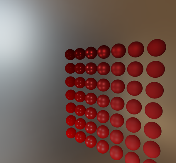
If it looks somewhat similar you've successfully pre-filtered the HDR environment map. Play around with different mipmap levels to see the pre-filter map gradually change from sharp to blurry reflections on increasing mip levels.
这看起来有点像HDR环境贴图的天空盒,证明你成功地得到了pre-filter贴图。用不同mkpmap层显示看看,pre-filter会逐渐从清晰到模糊。
Pre-filter卷积的瑕疵
While the current pre-filter map works fine for most purposes, sooner or later you'll come across several render artifacts that are directly related to the pre-filter convolution. I'll list the most common here including how to fix them.
尽管现在的pre-filter贴图在大多数时候工作得很好,早晚你会发现几个直接与pre-fitler有关的瑕疵。这里列举几个最常见的,并说明如何解决它们。
高粗糙度时的cubemap缝合线
Sampling the pre-filter map on surfaces with a rough surface means sampling the pre-filter map on some of its lower mip levels. When sampling cubemaps, OpenGL by default doesn't linearly interpolate across cubemap faces. Because the lower mip levels are both of a lower resolution and the pre-filter map is convoluted with a much larger sample lobe, the lack of between-cube-face filtering becomes quite apparent:
对更高粗糙度的表面采样意味着对更深的mipmap层采样。对cubemap采样时,OpenGL默认不在face之间线性插值。因为更深的mipmap层既是低分辨率,又是卷积了更大的采样叶,face之间的过滤损失变得十分明显。

Luckily for us, OpenGL gives us the option to properly filter across cubemap faces by enabling GL_TEXTURE_CUBE_MAP_SEAMLESS:
幸运的是,OpenGL给了我们选项,可以适当地在face之间过滤。只需启用:
glEnable(GL_TEXTURE_CUBE_MAP_SEAMLESS);
Simply enable this property somewhere at the start of your application and the seams will be gone.
在应用程序启动的时候,启用这个开关,缝合线就消失了。
Pre-fitler卷积中的亮点
Due to high frequency details and wildly varying light intensities in specular reflections, convoluting the specular reflections requires a large number of samples to properly account for the wildly varying nature of HDR environmental reflections. We already take a very large number of samples, but on some environments it might still not be enough at some of the rougher mip levels in which case you'll start seeing dotted patterns emerge around bright areas:
由于specular反射中的高频细节和广泛变化的强度,卷积需要很大的采样量。虽然如此,在比较粗糙的mipmap上仍旧不够,你会看到点状的模式出现在亮光区域:
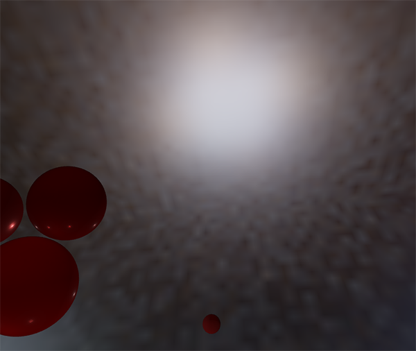
One option is to further increase the sample count, but this won't be enough for all environments. As described by Chetan Jags we can reduce this artifact by (during the pre-filter convolution) not directly sampling the environment map, but sampling a mip level of the environment map based on the integral's PDF and the roughness:
一个选择是增加采样量,但这对有的环境仍旧不够。如Chetan Jags所述,我们可以通过(在pre-filter卷积中)不直接对环境贴图采样来减少瑕疵,而是基于积分的pdf和粗糙度对环境贴图的一个mipmap层采样:
 float D   = DistributionGGX(NdotH, roughness);

 float pdf = (D * NdotH / (4.0 * HdotV)) + 0.0001;

 float resolution = 512.0; // resolution of source cubemap (per face)

 float saTexel  = 4.0 * PI / (6.0 * resolution * resolution);

 float saSample = 1.0 / (float(SAMPLE_COUNT) * pdf + 0.0001);

 float mipLevel = roughness == 0.0 ? 0.0 : 0.5 * log2(saSample / saTexel);
Don't forget to enable trilinear filtering on the environment map you want to sample its mip levels from:
别忘了启用三线过滤:
 glBindTexture(GL_TEXTURE_CUBE_MAP, envCubemap);

 glTexParameteri(GL_TEXTURE_CUBE_MAP, GL_TEXTURE_MIN_FILTER, GL_LINEAR_MIPMAP_LINEAR);
And let OpenGL generate the mipmaps after the cubemap's base texture is set:
在cubemap的第一个mipmap层完成之后生成后续的mipmap:
 // convert HDR equirectangular environment map to cubemap equivalent

 [...]

 // then generate mipmaps

 glBindTexture(GL_TEXTURE_CUBE_MAP, envCubemap);

 glGenerateMipmap(GL_TEXTURE_CUBE_MAP);
This works surprisingly well and should remove most, if not all, dots in your pre-filter map on rougher surfaces.
这工作得出人意料得好,能够移出大部分(或全部)pre-filter贴图中的粗糙表面的点现象。
预计算BRDF
With the pre-filtered environment up and running, we can focus on the second part of the split-sum approximation: the BRDF. Let's briefly review the specular split sum approximation again:
随着pre-fitler环境贴图上线运行,我们可以关注拆分求和近似的第二个部分:BRDF。我们简单地回忆一下拆分求和近似:

We've pre-computed the left part of the split sum approximation in the pre-filter map over different roughness levels. The right side requires us to convolute the BRDF equation over the angle n⋅ωo, the surface roughness and Fresnel's F0. This is similar to integrating the specular BRDF with a solid-white environment or a constant radiance Li of 1.0. Convoluting the BRDF over 3 variables is a bit much, but we can move F0 out of the specular BRDF equation:
我们已经预计算了左边的积分。右边的积分要求我们围绕角度n⋅ωo、粗糙度和菲涅耳尝试F0队BRDF卷积。这类似于对纯白色环境贴图或辐照度为常量1.0的BRDF积分。对3个变量卷积太难了,但我们可以把F0移到积分外面:

With F being the Fresnel equation. Moving the Fresnel denominator to the BRDF gives us the following equivalent equation:
其中F代表菲涅耳方程。将菲涅耳分母移到BRDF,得到:

Substituting the right-most F with the Fresnel-Schlick approximation gives us:
用Fresnel-Schlick近似代替右边的F,得到:

Let's replace (1−ωo⋅h)5 by α to make it easier to solve for F0:
我们用α代替(1−ωo⋅h)5,从而对收拾F0简单点:


Then we split the Fresnel function F over two integrals:
然后我们把菲涅耳方程F拆分为2个积分:

This way, F0 is constant over the integral and we can take F0 out of the integral. Next, we substitute α back to its original form giving us the final split sum BRDF equation:
这样,F0在积分上就是常量,我们可以将F0移出积分。下一步,我们将α替换回它原来的形式。现在就得到了最终的拆分求和BRDF方程:

The two resulting integrals represent a scale and a bias to F0 respectively. Note that as f(p,ωi,ωo) already contains a term for F they both cancel out, removing F from f.
这两个积分分别表示对F0的缩放和偏移。注意,由于f(p,ωi,ωo)已经包含了F项,他们抵消了,从f中移除了。
In a similar fashion to the earlier convoluted environment maps, we can convolute the BRDF equations on their inputs: the angle between n and ωo and the roughness, and store the convoluted result in a texture. We store the convoluted results in a 2D lookup texture (LUT) known as a BRDF integration map that we later use in our PBR lighting shader to get the final convoluted indirect specular result.
类似之前的卷积操作,我们可以针对BRDF的输入参数进行卷积:n和ωo之间的角度,以及粗糙度。然后将结果保存到贴图中。我们将卷积结果保存到一个二维查询纹理(LUT),即BRDF积分贴图,稍后用于PBR光照shader,得到最终的非直接specular光照结果。
The BRDF convolution shader operates on a 2D plane, using its 2D texture coordinates directly as inputs to the BRDF convolution (NdotV and roughness). The convolution code is largely similar to the pre-filter convolution, except that it now processes the sample vector according to our BRDF's geometry function and Fresnel-Schlick's approximation:
BRDF卷积shader在二维平面上工作,它使用二维纹理坐标直接作为输入参数,以此卷积BRDF(NdotV 和roughness)。卷积代码和pre-filter卷积很相似,除了它现在根据几何函数G和Fresnel-Schlick近似来处理采样限量:
 vec2 IntegrateBRDF(float NdotV, float roughness)

 {

     vec3 V;

     V.x = sqrt(1.0 - NdotV*NdotV);

     V.y = 0.0;

     V.z = NdotV;

     float A = 0.0;

     float B = 0.0;

     vec3 N = vec3(0.0, 0.0, 1.0);

     const uint SAMPLE_COUNT = 1024u;

     for(uint i = 0u; i < SAMPLE_COUNT; ++i)

     {

         vec2 Xi = Hammersley(i, SAMPLE_COUNT);

         vec3 H  = ImportanceSampleGGX(Xi, N, roughness);

         vec3 L  = normalize(2.0 * dot(V, H) * H - V);

         float NdotL = max(L.z, 0.0);

         float NdotH = max(H.z, 0.0);

         float VdotH = max(dot(V, H), 0.0);

         if(NdotL > 0.0)

         {

             float G = GeometrySmith(N, V, L, roughness);

             float G_Vis = (G * VdotH) / (NdotH * NdotV);

             float Fc = pow(1.0 - VdotH, 5.0);

             A += (1.0 - Fc) * G_Vis;

             B += Fc * G_Vis;

         }

     }

     A /= float(SAMPLE_COUNT);

     B /= float(SAMPLE_COUNT);

     return vec2(A, B);

 }

 // ----------------------------------------------------------------------------

 void main()

 {

     vec2 integratedBRDF = IntegrateBRDF(TexCoords.x, TexCoords.y);

     FragColor = integratedBRDF;

 }
IntegrateBRDF
As you can see the BRDF convolution is a direct translation from the mathematics to code. We take both the angle θ and the roughness as input, generate a sample vector with importance sampling, process it over the geometry and the derived Fresnel term of the BRDF, and output both a scale and a bias to F0 for each sample, averaging them in the end.
你可以看到,BRDF卷积就是直接把数学公式转换为代码。我们以角度θ和粗糙度为输入参数,用重要性采样方法生成采样向量,用几何函数G和菲涅耳项处理它,输出F0的缩放和偏移量,最后求平均值。
You might've recalled from the theory tutorial that the geometry term of the BRDF is slightly different when used alongside IBL as its k variable has a slightly different interpretation:
你可能回想起在理论教程中,BRDF的几何函数项在用于IBL时有所不同,k变量的解释是不同的:
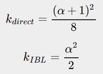
Since the BRDF convolution is part of the specular IBL integral we'll use kIBL for the Schlick-GGX geometry function:
既然BRDF卷积是specular的IBL的一部分,我们将在几何函数中用kIBL这个解释:
 float GeometrySchlickGGX(float NdotV, float roughness)

 {

     float a = roughness;

     float k = (a * a) / 2.0;

     float nom   = NdotV;

     float denom = NdotV * (1.0 - k) + k;

     return nom / denom;

 }

 // ----------------------------------------------------------------------------

 float GeometrySmith(vec3 N, vec3 V, vec3 L, float roughness)

 {

     float NdotV = max(dot(N, V), 0.0);

     float NdotL = max(dot(N, L), 0.0);

     float ggx2 = GeometrySchlickGGX(NdotV, roughness);

     float ggx1 = GeometrySchlickGGX(NdotL, roughness);

     return ggx1 * ggx2;

 }
Note that while k takes a as its parameter we didn't square roughness as a as we originally did for other interpretations of a; likely as a is squared here already. I'm not sure whether this is an inconsistency on Epic Games' part or the original Disney paper, but directly translating roughness to a gives the BRDF integration map that is identical to Epic Games' version.
注意,尽管k以a为输入参数,我们没有将roughness 的平方作为a,我们之前却是这么做的。可能这里的a已经平方过了。我不确定这是Epic游戏公司的不一致性,还是最初的Disney文献的问题,但是直接将roughness 传递给a,确实得到了与Epic游戏公司相同的BRDF积分贴图。
Finally, to store the BRDF convolution result we'll generate a 2D texture of a 512 by 512 resolution.
最后,为保存BRDF卷积结果,我们创建一个二维纹理,尺寸为512x512:
 unsigned int brdfLUTTexture;

 glGenTextures(, &brdfLUTTexture);

 // pre-allocate enough memory for the LUT texture.

 glBindTexture(GL_TEXTURE_2D, brdfLUTTexture);

 glTexImage2D(GL_TEXTURE_2D, , GL_RG16F, , , , GL_RG, GL_FLOAT, );

 glTexParameteri(GL_TEXTURE_2D, GL_TEXTURE_WRAP_S, GL_CLAMP_TO_EDGE);

 glTexParameteri(GL_TEXTURE_2D, GL_TEXTURE_WRAP_T, GL_CLAMP_TO_EDGE);

 glTexParameteri(GL_TEXTURE_2D, GL_TEXTURE_MIN_FILTER, GL_LINEAR);

 glTexParameteri(GL_TEXTURE_2D, GL_TEXTURE_MAG_FILTER, GL_LINEAR);
Note that we use a 16-bit precision floating format as recommended by Epic Games. Be sure to set the wrapping mode to GL_CLAMP_TO_EDGE to prevent edge sampling artifacts.
注意,我们使用16位精度浮点数格式,这是Epic游戏公司推荐的。确保wrapping模式为GL_CLAMP_TO_EDGE ,防止边缘采样瑕疵。
Then, we re-use the same framebuffer object and run this shader over an NDC screen-space quad:
然后,我们复用相同的Framebuffer对象,在NDC空间(画一个铺满屏幕的四边形)运行下面的shader:
 glBindFramebuffer(GL_FRAMEBUFFER, captureFBO);

 glBindRenderbuffer(GL_RENDERBUFFER, captureRBO);

 glRenderbufferStorage(GL_RENDERBUFFER, GL_DEPTH_COMPONENT24, , );

 glFramebufferTexture2D(GL_FRAMEBUFFER, GL_COLOR_ATTACHMENT0, GL_TEXTURE_2D, brdfLUTTexture, );

 glViewport(, , , );

 brdfShader.use();

 glClear(GL_COLOR_BUFFER_BIT | GL_DEPTH_BUFFER_BIT);

 RenderQuad();

 glBindFramebuffer(GL_FRAMEBUFFER, );
The convoluted BRDF part of the split sum integral should give you the following result:
拆分求和积分的BRDF部分的卷积会得到如下图所示的结果:

With both the pre-filtered environment map and the BRDF 2D LUT we can re-construct the indirect specular integral according to the split sum approximation. The combined result then acts as the indirect or ambient specular light.
有了pre-filter环境贴图和BRDF的二维LUT贴图,我们可以根据拆分求和近似来重构非直接specular积分。相乘的结果就是非直接或环境specular光。
IBL反射完成
To get the indirect specular part of the reflectance equation up and running we need to stitch both parts of the split sum approximation together. Let's start by adding the pre-computed lighting data to the top of our PBR shader:
为了让反射率方程中的非直接specular部分上线运行,我们需要将拆分求和近似的两部分钉在一起。开始时,让我们把预计算的光照数据放到PBR shaer的开头:
 uniform samplerCube prefilterMap;

 uniform sampler2D   brdfLUT;
First, we get the indirect specular reflections of the surface by sampling the pre-filtered environment map using the reflection vector. Note that we sample the appropriate mip level based on the surface roughness, giving rougher surfaces blurrierspecular reflections.
首先,使用反射向量,通过对pre-filter环境贴图采样,我们得到表面的非直接specular反射强度。注意,我们根据表面的粗糙度度对最接近的mipmap层采样,这会让更粗糙的表面表现出更模糊的反射效果。
 void main()

 {

     [...]

     vec3 R = reflect(-V, N);

     const float MAX_REFLECTION_LOD = 4.0;

     vec3 prefilteredColor = textureLod(prefilterMap, R,  roughness * MAX_REFLECTION_LOD).rgb;

     [...]

 }
In the pre-filter step we only convoluted the environment map up to a maximum of 5 mip levels (0 to 4), which we denote here as MAX_REFLECTION_LOD to ensure we don't sample a mip level where there's no (relevant) data.
在pre-tilter步骤中我们只卷积了5个mipmap层(0-4),我们这里用MAX_REFLECTION_LOD 确保不对没有数据的位置采样。
Then we sample from the BRDF lookup texture given the material's roughness and the angle between the normal and view vector:
给定材质的粗糙度和角度(法线和观察者之间的角度),我们从BRDF的查询纹理中采样:
 vec3 F        = FresnelSchlickRoughness(max(dot(N, V), 0.0), F0, roughness);

 vec2 envBRDF  = texture(brdfLUT, vec2(max(dot(N, V), 0.0), roughness)).rg;

 vec3 specular = prefilteredColor * (F * envBRDF.x + envBRDF.y);
Given the scale and bias to F0 (here we're directly using the indirect Fresnel result F) from the BRDF lookup texture we combine this with the left pre-filter portion of the IBL reflectance equation and re-construct the approximated integral result as specular.
从BRDF的查询纹理中找到了F0的缩放和偏移(这里我们直接使用了非直接菲涅耳函数F),我们联合IBL反射率方程左边的pre-filter部分,重构出specular的近似积分值。
This gives us the indirect specular part of the reflectance equation. Now, combine this with the diffuse part of the reflectance equation from the last tutorial and we get the full PBR IBL result:
这就得到了反射率方程的非直接specular部分。现在,联合反射率方程的diffuse部分(从上一篇教程中)我们就得到了PBR全部的IBL结果:
 vec3 F = FresnelSchlickRoughness(max(dot(N, V), 0.0), F0, roughness);

 vec3 kS = F;

 vec3 kD = 1.0 - kS;

 kD *= 1.0 - metallic;

 vec3 irradiance = texture(irradianceMap, N).rgb;

 vec3 diffuse    = irradiance * albedo;

 const float MAX_REFLECTION_LOD = 4.0;

 vec3 prefilteredColor = textureLod(prefilterMap, R,  roughness * MAX_REFLECTION_LOD).rgb;

 vec2 envBRDF  = texture(brdfLUT, vec2(max(dot(N, V), 0.0), roughness)).rg;

 vec3 specular = prefilteredColor * (F * envBRDF.x + envBRDF.y);

 vec3 ambient = (kD * diffuse + specular) * ao;
Note that we don't multiply specular by kS as we already have a Fresnel multiplication in there.
注意,我们没有用kS 乘以specular ,因为我们这里已经有个菲涅耳乘过了。
Now, running this exact code on the series of spheres that differ by their roughness and metallic properties we finally get to see their true colors in the final PBR renderer:
现在,运行本系列教程中不同粗糙度和金属度球体的那个代码,我们最终得以看它们在PBR渲染下的真正颜色:
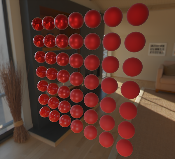
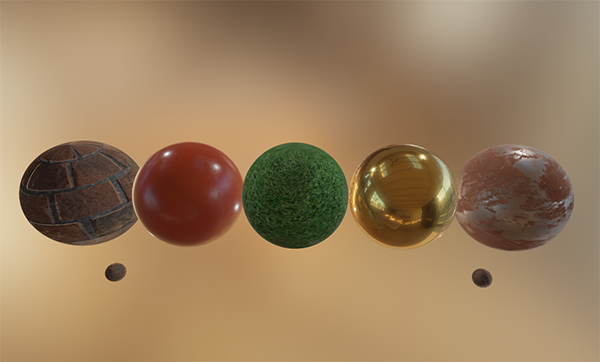
We could even go wild, and use some cool textured PBR materials:
我们还可以更疯狂点,用一些酷炫的纹理(来自PBR materials):
Or load this awesome free PBR 3D model by Andrew Maximov:
或者加载这个棒棒的免费PBR三维模型(Andrew Maximov所做):
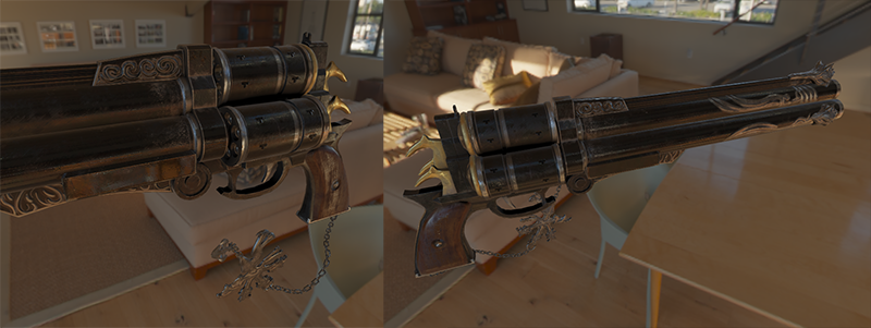
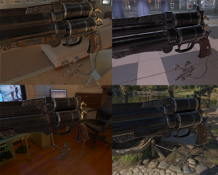
I'm sure we can all agree that our lighting now looks a lot more convincing. What's even better, is that our lighting looks physically correct, regardless of which environment map we use. Below you'll see several different pre-computed HDR maps, completely changing the lighting dynamics, but still looking physically correct without changing a single lighting variable!
我确定我们都同意这一点:我们的光照现在看起来真实得多了。更好的是,我们的光照是物理正确的,无论我们用那个环境贴图。下面你将看到几个不同的预计算的HDR贴图,完全改变了光照效果,但是仍旧是看起来物理正确的。这不需要改变一丢丢光照参数!
Well, this PBR adventure turned out to be quite a long journey. There are a lot of steps and thus a lot that could go wrong so carefully work your way through the sphere scene or textured scene code samples (including all shaders) if you're stuck, or check and ask around in the comments.
此次PBR探险之旅最终显得相当漫长。有很多步骤,所以有很多可能出错的地方,所以,如果卡住了,仔细小心地检查sphere scene 或textured scene代码(包括所有的shader),或者检查下注释。
接下来?
Hopefully, by the end of this tutorial you should have a pretty clear understanding of what PBR is about, and even have an actual PBR renderer up and running. In these tutorials, we've pre-computed all the relevant PBR image-based lighting data at the start of our application, before the render loop. This was fine for educational purposes, but not too great for any practical use of PBR. First, the pre-computation only really has to be done once, not at every startup. And second, the moment you use multiple environment maps you'll have to pre-compute each and every one of them at every startup which tends to build up.
但愿,在本教程结束时你已经对PBR有了很清除的理解,甚至有了可能实际运行起来的渲染器。这些教程中,我们在程序开始时预计算了所有相关的IBL数据,然后启动渲染循环。这对教程是没问题的,但是对任何实际应用的软件是不可行的。首先,预计算只需要完成一次,不需要每次启动都做。其次,使用多环境贴图时,你不得不每次都把它们全算一遍,这太浪费了。
For this reason you'd generally pre-compute an environment map into an irradiance and pre-filter map just once, and then store it on disk (note that the BRDF integration map isn't dependent on an environment map so you only need to calculate or load it once). This does mean you'll need to come up with a custom image format to store HDR cubemaps, including their mip levels. Or, you'll store (and load) it as one of the available formats (like .dds that supports storing mip levels).
因此,你应该将预计算结果保存到硬盘上(注意BRDF积分贴图不依赖环境贴图,所以你只需计算和加载一次)。这意味着你需要找一个自定义的图片格式来存储HDR的cubemap,包括它们的各个mipmap层。或者,你用现有的格式(比如*.dss支持保存多个mipmap层)。
Furthermore, we've described the total process in these tutorials, including generating the pre-computed IBL images to help further our understanding of the PBR pipeline. But, you'll be just as fine by using several great tools like cmftStudio or IBLBaker to generate these pre-computed maps for you.
此外,我们在教程中描述了预计算的所有过程,这是为了加深对PBR管道的理解。你完全可以用一些棒棒的工具(例如cmftStudio 或IBLBaker )来为你完成这些预计算。
One point we've skipped over is pre-computed cubemaps as reflection probes: cubemap interpolation and parallax correction. This is the process of placing several reflection probes in your scene that take a cubemap snapshot of the scene at that specific location, which we can then convolute as IBL data for that part of the scene. By interpolating between several of these probes based on the camera's vicinity we can achieve local high-detail image-based lighting that is simply limited by the amount of reflection probes we're willing to place. This way, the image-based lighting could correctly update when moving from a bright outdoor section of a scene to a darker indoor section for instance. I'll write a tutorial about reflection probes somewhere in the future, but for now I recommend the article by Chetan Jags below to give you a head start.
我们跳过的一个点,是将预计算的cubemap用作反射探针:cubemap插值和视差校正。这个说的是,在你的场景中放置几个反射探针,它们在各自的位置拍个cubemap快照,卷积为IBL数据,用作场景中那一部分的光照计算。通过在camera最近的几个探针间插值,我们可以实现局部高细节度的IBL光照(只要我们愿意放置够多的探针)。这样,当从一个明亮的门外部分移动到比较暗的门内部分时,IBL光照可以正确地更新。未来我将写一篇关于探针的教程,但是现在我推荐下面Chetan Jags的文章,你可以从此开始。
更多阅读
- Real Shading in Unreal Engine 4: explains Epic Games' split sum approximation. This is the article the IBL PBR code is based of.
- 解释了Epic游戏公司的拆分求和近似方案。本文基于此而作。
- Physically Based Shading and Image Based Lighting: great blog post by Trent Reed about integrating specular IBL into a PBR pipeline in real time.
- 了不起的Trent Reed的博客,关于实时的将BL集成进PBR管道。
- Image Based Lighting: very extensive write-up by Chetan Jags about specular-based image-based lighting and several of its caveats, including light probe interpolation.
- 由Chetan Jags广泛评论的基于specular和IBL的光照及其警告,包括光探针插值。
- Moving Frostbite to PBR: well written and in-depth overview of integrating PBR into a AAA game engine by Sébastien Lagarde and Charles de Rousiers.
- 由bastien Lagarde和Charles de Rousiers编写的深度好文,探讨了如何将PBR集成到AAA游戏引擎。
- Physically Based Rendering – Part Three: high level overview of IBL lighting and PBR by the JMonkeyEngine team.
- 由JMonkeyEngine小组提供的IBL光照和PBR高层概览。
- Implementation Notes: Runtime Environment Map Filtering for Image Based Lighting: extensive write-up by Padraic Hennessy about pre-filtering HDR environment maps and significanly optimizing the sample process.
- 由Padraic Hennessy的评论,关于pre-filter的HDR环境贴图及其高度优化。
CSharpGL(54)用基于图像的光照(IBL)来计算PBR的Specular部分的更多相关文章
- 相似图像识别检 —基于图像签名(LSH)
原文链接:http://grunt1223.iteye.com/blog/828192 参考:人工智能,一种现代方法 第 617页,且原始论文给出了完整的证明过程.在ANN方法中,LSH算一种可靠的紧 ...
- Unity——基于ShaderLab实现光照系统
这篇主要总结Unity中ShaderLab的着色器代码实现总结,需要有一定图形学基础和ShaderLab基础: 一.着色器 1.顶点片元着色器 分顶点着色器和片元着色器,对应渲染管线的顶点变换和片元着 ...
- python爬虫(正则取数据)读取表格内的基金代码后爬取基金最新净值,同时写到对应的表格中,基于最近一次购买净值计算出涨跌幅(名字有点长)
最近基金跌的真够猛,虽说是定投,但大幅度下跌,有时候适当的增加定投数也是降低平均成本的一种方式 每天去看去算太费时间,写了个爬虫,让他自动抓数据后自动计算出来吧 实现逻辑: 1.创建了一个excel表 ...
- 个人翻译的cedec2010基于物理的光照
作为自己介绍基于物理渲染计划的一部分,在自己总结和发布的同时,也会翻译一些国外的优秀资料做推广 本文是Tri Ace 在 cedec2010上发布的文章,主要描述了他们基于物理光照的实现方法,这 ...
- 基于图像二维熵的视频信号丢失检测(Signal Loss Detection)
1 图像二维熵 图像二维熵作为一种特征评价尺度能够反映出整个图像所含平均信息量的高低,熵值(H)越大则代表图像所包含的信息越多,反之熵值(H)越小,则图像包含的信息越少.对于图像信息量,可以简单地认 ...
- 基于图像切换器(imageSwitcher)的支持动画的图片浏览器
利用GridView和ImageSwitcher的基本用法 public class MainActivity extends Activity { int[] imageIds = new int[ ...
- 使用Python实现基于图像识别的iOS自动化测试
相对于Android来说,iOS比较封闭.这一点,在设计和评估自动化测试方案的时候感觉尤其强烈.iOS平台上没有特别好用的自动化测试工具.苹果针对iOS提供了UI Automation的Instrum ...
- (数据科学学习手札84)基于geopandas的空间数据分析——空间计算篇(上)
本文示例代码.数据及文件已上传至我的Github仓库https://github.com/CNFeffery/DataScienceStudyNotes 1 简介 在本系列之前的文章中我们主要讨论了g ...
- 基于案例贯通 Spark Streaming 流计算框架的运行源码
本期内容 : Spark Streaming+Spark SQL案例展示 基于案例贯穿Spark Streaming的运行源码 一. 案例代码阐述 : 在线动态计算电商中不同类别中最热门的商品排名,例 ...
随机推荐
- ActiveMQ下载与安装(消息中间件JMS)
下载 官方网站下载:http://activemq.apache.org/ 1.3.2安装(Linux) (1)将apache-activemq-5.12.0-bin.tar.gz 上传至服务器 (2 ...
- 2019/12/13学习内容摘要(Linux磁盘管理①)
一,查看磁盘或目录容量 1.命令df 查看已挂载磁盘的总容量,使用容量,剩余容量等,可以不加任何参数,默认以KB为单位 选项[-i] 表示查看inodes的使用情况 [-h] 表示用合适的单位显示 ...
- MQ脚本回放报错2059
1.响应2059错误 1.1. 涉及协议 MQ,调试回放阶段 1.2. 错误信息 完成码2原因为2059:未能为 '10.200.100.75:QMEMBFE' 创建 MQQueueManag ...
- 2019-2020-1 20199305《Linux内核原理与分析》第十二周作业
缓冲区溢出漏洞实验 (一)何为缓冲区溢出漏洞 缓冲区溢出是指程序试图向缓冲区写入超出预分配固定长度数据的情况.这一漏洞可以被恶意用户利用来改变程序的流控制,甚至执行代码的任意片段.这一漏洞的出现是由于 ...
- CMKAE简单实用指南
CMake is an open-source, cross-platform family of tools designed to build, test and package software ...
- appium元素定位之AndroidUiAutomator
UIAutomator 元素定位是 Android 系统原生支持的定位方式,虽然与 xpath 类似,但比它更好用,并且支持元素全部的属性定位,定位原理是通过 android 自带的android u ...
- 软件测试价值提升之路- 第三章"拦截缺陷 "读书笔记
作为一个测试团队,基本的职责是:测试产品,发现缺陷,报告结果,使每个版本的测试水准稳步提升.这些价值是作为一个测试所必须具备的,发挥这些价值能够让测试获得研发团队的基本信任.这类价值分为3部分: 1) ...
- PostgreSQL数据库一些tricks
PostgreSQL自带Pgadmin客户端,可用于访问本地和远程PG库,一些tricks如下: 1.联合查询 SELECT * FROM table1 INNER JOIN table2 ON ta ...
- Java描述设计模式(12):外观模式
本文源码:GitHub·点这里 || GitEE·点这里 一.生活场景 1.场景描述 在移动互联网没有普及之前,去饭店吃饭的流程大致如下:选座位,排队,点菜,结账.后来移动互联网普及,通过手机APP就 ...
- [Spring cloud 一步步实现广告系统] 8. 检索系统配置&依赖
工作流程 项目依赖 <dependencies> <!-- hystrix 监控面板 --> <dependency> <groupId>org.spr ...
