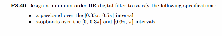
《DSP using MATLAB》Problem 8.46

下雨了，大风降温，一地树叶，终于进入冬季了

代码：

%% ------------------------------------------------------------------------
%%            Output Info about this m-file
fprintf('\n***********************************************************\n');
fprintf('        <DSP using MATLAB> Problem 8.46.4 \n\n');
 
banner();
%% ------------------------------------------------------------------------
 
% Digital Filter Specifications:   Elliptic bandpass
wsbp = [0.30*pi 0.60*pi];             % digital stopband freq in rad
wpbp = [0.35*pi 0.50*pi];             % digital passband freq in rad
  Rp = 1.00;                          % passband ripple in dB
  As = 40;                            % stopband attenuation in dB
 
Ripple = 10 ^ (-Rp/20)           % passband ripple in absolute
Attn = 10 ^ (-As/20)             % stopband attenuation in absolute
 
fprintf('\n*******Digital bandpass, Coefficients of DIRECT-form***********\n');
[bbp, abp] = elipbpf(wpbp, wsbp, Rp, As)
[C, B, A] = dir2cas(bbp, abp)
 
% Calculation of Frequency Response:
[dbbp, magbp, phabp, grdbp, wwbp] = freqz_m(bbp, abp);
 
% ---------------------------------------------------------------
%    find Actual Passband Ripple and Min Stopband attenuation
% ---------------------------------------------------------------
delta_w = 2*pi/1000;
Rp_bp = -(min(dbbp(ceil(wpbp(1)/delta_w+1):1:ceil(wpbp(2)/delta_w+1))));      % Actual Passband Ripple
 
fprintf('\nActual Passband Ripple is %.4f dB.\n', Rp_bp);
 
As_bp = -round(max(dbbp(1:1:ceil(wsbp(1)/delta_w)+1)));                    % Min Stopband attenuation
fprintf('\nMin Stopband attenuation is %.4f dB.\n\n', As_bp);
 
%% -----------------------------------------------------------------
%%                             Plot
%% -----------------------------------------------------------------  
 
figure('NumberTitle', 'off', 'Name', 'Problem 8.46.4 Elliptic bp by elipbpf function')
set(gcf,'Color','white');
M = 1;                          % Omega max
 
subplot(2,2,1); plot(wwbp/pi, magbp); axis([0, M, 0, 1.2]); grid on;
xlabel('Digital frequency in \pi units'); ylabel('|H|'); title('Magnitude Response');
set(gca, 'XTickMode', 'manual', 'XTick', [0, 0.3, 0.35, 0.5, 0.6, M]);
set(gca, 'YTickMode', 'manual', 'YTick', [0, 0.01, 0.8913, 1]);
 
subplot(2,2,2); plot(wwbp/pi, dbbp); axis([0, M, -100, 2]); grid on;
xlabel('Digital frequency in \pi units'); ylabel('Decibels'); title('Magnitude in dB');
set(gca, 'XTickMode', 'manual', 'XTick', [0, 0.3, 0.35, 0.5, 0.6, M]);
set(gca, 'YTickMode', 'manual', 'YTick', [-80, -40, -1, 0]);
set(gca,'YTickLabelMode','manual','YTickLabel',['80'; '40';'1 ';' 0']);
 
subplot(2,2,3); plot(wwbp/pi, phabp/pi); axis([0, M, -1.1, 1.1]); grid on;
xlabel('Digital frequency in \pi nuits'); ylabel('radians in \pi units'); title('Phase Response');
set(gca, 'XTickMode', 'manual', 'XTick', [0, 0.3, 0.35, 0.5, 0.6, M]);
set(gca, 'YTickMode', 'manual', 'YTick', [-1:0.5:1]);
 
subplot(2,2,4); plot(wwbp/pi, grdbp); axis([0, M, 0, 80]); grid on;
xlabel('Digital frequency in \pi units'); ylabel('Samples'); title('Group Delay');
set(gca, 'XTickMode', 'manual', 'XTick', [0, 0.3, 0.35, 0.5, 0.6, M]);
set(gca, 'YTickMode', 'manual', 'YTick', [0:20:80]);
 
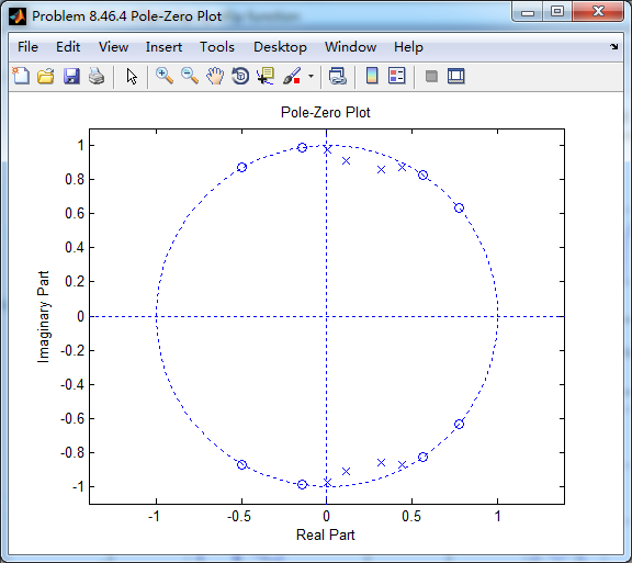
figure('NumberTitle', 'off', 'Name', 'Problem 8.46.4 Pole-Zero Plot')
set(gcf,'Color','white');
zplane(bbp, abp);
title(sprintf('Pole-Zero Plot'));
%pzplotz(b,a);
 
% -----------------------------------------------------
%              method 3  elip function
% -----------------------------------------------------
 
% Calculation of Elliptic filter parameters:
[N, wn] = ellipord(wpbp/pi, wsbp/pi, Rp, As);
 
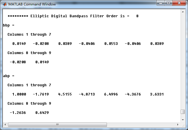
fprintf('\n  ********* Elliptic Digital Bandpass Filter Order is = %3.0f \n', 2*N)
 
% Digital Elliptic Bandpass Filter Design:
[bbp, abp] = ellip(N, Rp, As, wn)
 
[C, B, A] = dir2cas(bbp, abp)
 
% Calculation of Frequency Response:
[dbbp, magbp, phabp, grdbp, wwbp] = freqz_m(bbp, abp);
 
% ---------------------------------------------------------------
%    find Actual Passband Ripple and Min Stopband attenuation
% ---------------------------------------------------------------
delta_w = 2*pi/1000;
Rp_bp = -(min(dbbp(ceil(wpbp(1)/delta_w+1):1:ceil(wpbp(2)/delta_w+1))));      % Actual Passband Ripple
 
fprintf('\nActual Passband Ripple is %.4f dB.\n', Rp_bp);
 
As_bp = -round(max(dbbp(1:1:ceil(wsbp(1)/delta_w)+1)));                    % Min Stopband attenuation
fprintf('\nMin Stopband attenuation is %.4f dB.\n\n', As_bp);
 
%% -----------------------------------------------------------------
%%                             Plot
%% -----------------------------------------------------------------  
 
figure('NumberTitle', 'off', 'Name', 'Problem 8.46.4 Elliptic bp by ellip function')
set(gcf,'Color','white');
M = 1;                          % Omega max
 
subplot(2,2,1); plot(wwbp/pi, magbp); axis([0, M, 0, 1.2]); grid on;
xlabel('Digital frequency in \pi units'); ylabel('|H|'); title('Magnitude Response');
set(gca, 'XTickMode', 'manual', 'XTick', [0, 0.3, 0.35, 0.5, 0.6, M]);
set(gca, 'YTickMode', 'manual', 'YTick', [0, 0.01, 0.8913, 1]);
 
subplot(2,2,2); plot(wwbp/pi, dbbp); axis([0, M, -100, 2]); grid on;
xlabel('Digital frequency in \pi units'); ylabel('Decibels'); title('Magnitude in dB');
set(gca, 'XTickMode', 'manual', 'XTick', [0, 0.3, 0.35, 0.5, 0.6, M]);
set(gca, 'YTickMode', 'manual', 'YTick', [-80, -40, -1, 0]);
set(gca,'YTickLabelMode','manual','YTickLabel',['80'; '40';'1 ';' 0']);
 
subplot(2,2,3); plot(wwbp/pi, phabp/pi); axis([0, M, -1.1, 1.1]); grid on;
xlabel('Digital frequency in \pi nuits'); ylabel('radians in \pi units'); title('Phase Response');
set(gca, 'XTickMode', 'manual', 'XTick', [0, 0.3, 0.35, 0.5, 0.6, M]);
set(gca, 'YTickMode', 'manual', 'YTick', [-1:0.5:1]);
 
subplot(2,2,4); plot(wwbp/pi, grdbp); axis([0, M, 0, 100]); grid on;
xlabel('Digital frequency in \pi units'); ylabel('Samples'); title('Group Delay');
set(gca, 'XTickMode', 'manual', 'XTick', [0, 0.3, 0.35, 0.5, 0.6, M]);
set(gca, 'YTickMode', 'manual', 'YTick', [0:30:90]);

　　运行结果：

看题目，是Elliptic型数字带通，设计指标，DB转换成绝对指标

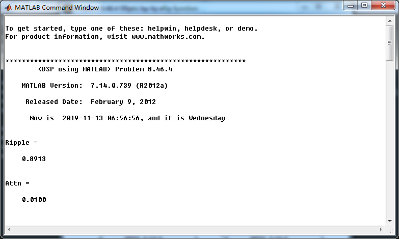
Elliptic模拟低通原型阶数是4，使用elipbpf函数设计带通，系统函数直接形式和串联形式的系数如下，

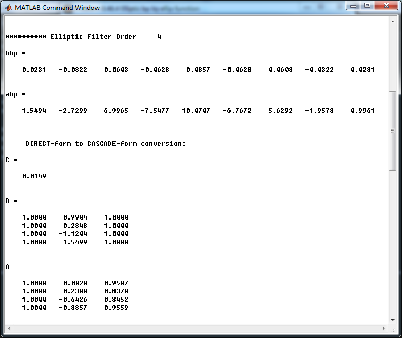
幅度谱、相位谱和群延迟响应

零极点图

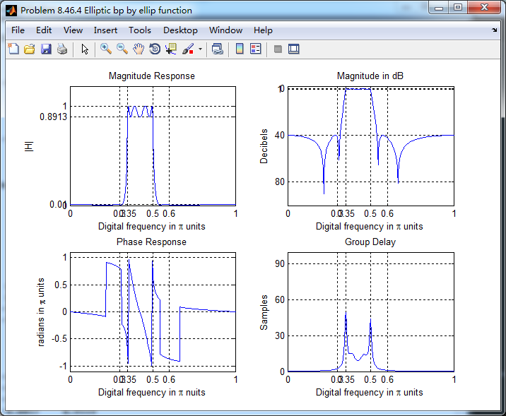
采用elip函数（MATLAB工具箱函数），设计带通，阶数是8阶，系统函数直接形式和串联形式的系数如下

幅度谱、相位谱和群延迟响应

给定通带、阻带衰减处的精确频带边界频率，我暂时不会计算，以后学会了再放图吧。