LogisticRegression in MLLib

例子

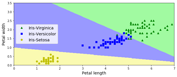
iris数据训练Logistic模型。特征petal width和petal height，分类目标有三类。

import org.apache.spark.mllib.classification.LogisticRegressionWithLBFGS
import org.apache.spark.mllib.evaluation.MulticlassMetrics
import org.apache.spark.mllib.linalg.Vectors
import org.apache.spark.mllib.regression.LabeledPoint
import org.apache.spark.rdd.RDD
import org.apache.spark.sql.SparkSession
object Test1 extends App {
  val spark = SparkSession
    .builder
    .appName("StructuredNetworkWordCountWindowed")
    .master("local[3]")
    .config("spark.sql.shuffle.partitions", 3)
    .config("spark.sql.autoBroadcastJoinThreshold", 1)
    .getOrCreate()
  spark.sparkContext.setLogLevel("INFO")
  val sc = spark.sparkContext
  val data: RDD[LabeledPoint] = sc.textFile("iris.txt").map { line =>
    val linesp = line.split("\\s+")
    LabeledPoint(linesp(2).toInt, Vectors.dense(linesp(0).toDouble, linesp(1).toDouble))
  }
  // Split data into training (60%) and test (40%).
  val splits = data.randomSplit(Array(0.6, 0.4), seed = 11L)
  val training = splits(0).cache()
  val test = splits(1)
  // Run training algorithm to build the model
  val model = new LogisticRegressionWithLBFGS()
    .setIntercept(true)
    .setNumClasses(3)
    .run(training)
  // Compute raw scores on the test set.
  val predictionAndLabels = test.map { case LabeledPoint(label, features) =>
    val prediction = model.predict(features)
    (prediction, label)
  }
  // Get evaluation metrics.
  val metrics = new MulticlassMetrics(predictionAndLabels)
  val accuracy = metrics.accuracy
  println(s"Accuracy = $accuracy")
}

训练结果

Accuracy = 0.9516129032258065
model : org.apache.spark.mllib.classification.LogisticRegressionModel: intercept = 0.0, numFeatures = 6, numClasses = 3, threshold = 0.5
weights = [10.806033250918638,59.0125055499883,-74.5967318848371,15.249528477342315,72.68333443959429,-119.02776352645247]

模型将特征空间划分结果（画图代码参见 http://www.cnblogs.com/luweiseu/p/7826679.html）：

ML LogisticRegress算法

算法流程在：

org.apache.spark.ml.classification.LogisticRegression
protected[org.apache.spark] def train(dataset: Dataset[_],
                                      handlePersistence: Boolean): LogisticRegressionModel

主要算法在：

val costFun = new LogisticCostFun(instances, numClasses, $(fitIntercept),
          $(standardization), bcFeaturesStd, regParamL2, multinomial = isMultinomial,
          $(aggregationDepth))

LogisticCostFun 实现了Breeze's DiffFunction[T]函数，计算multinomial (softmax) logistic loss

function, as used in multi-class classification (it is also used in binary logistic regression).

It returns the loss and gradient with L2 regularization at a particular point (coefficients).

该函数分布式计算参数梯度矩阵和损失

val logisticAggregator = {
      // 每个训练数据instance参与计算梯度矩阵
      val seqOp = (c: LogisticAggregator, instance: Instance) => c.add(instance)
      // 各个partition的aggregator merge
      val combOp = (c1: LogisticAggregator, c2: LogisticAggregator) => c1.merge(c2)
      // spark聚合调用
      instances.treeAggregate(
        new LogisticAggregator(bcCoeffs, bcFeaturesStd, numClasses, fitIntercept,
          multinomial)
      )(seqOp, combOp, aggregationDepth)
    }

Breeze凸优化：

LogisticCostFun 作为Breeze的凸优化模块（例如LBFGSB）的参数，计算最优的参数结果：

val states = optimizer.iterations(new CachedDiffFunction(costFun),
          new BDV[Double](initialCoefWithInterceptMatrix.toArray))

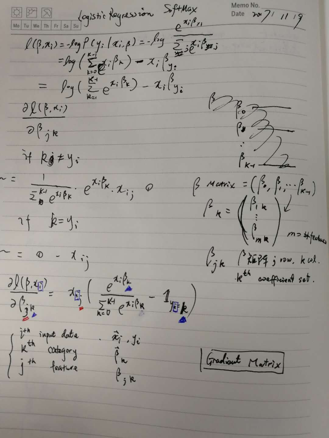
LogisticCostFun 梯度计算(LogisticAggregator)

该模块包含了LogisticRegression训练多类分类器时迭代（online）的逻辑。

主要逻辑是给定一个训练样本\(x_i\)，计算该样本对梯度矩阵中各个元素\(\beta_{j,k}\)的贡献。

LogisticAggregator computes the gradient and loss for binary or multinomial logistic (softmax)

loss function, as used in classification for instances in sparse or dense vector in an online

fashion.

Two LogisticAggregators can be merged together to have a summary of loss and gradient of

the corresponding joint dataset.

For improving the convergence rate during the optimization process and also to prevent against

features with very large variances exerting an overly large influence during model training,

packages like R's GLMNET perform the scaling to unit variance and remove the mean in order to

reduce the condition number. The model is then trained in this scaled space, but returns the

coefficients in the original scale. See page 9 in

http://cran.r-project.org/web/packages/glmnet/glmnet.pdf

However, we don't want to apply the [[org.apache.spark.ml.feature.StandardScaler]] on the

training dataset, and then cache the standardized dataset since it will create a lot of overhead.

As a result, we perform the scaling implicitly when we compute the objective function (though

we do not subtract the mean).

Note that there is a difference between multinomial (softmax) and binary loss. The binary case

uses one outcome class as a "pivot" and regresses the other class against the pivot. In the

multinomial case, the softmax loss function is used to model each class probability

independently. Using softmax loss produces K sets of coefficients, while using a pivot class

produces K - 1 sets of coefficients (a single coefficient vector in the binary case). In the

binary case, we can say that the coefficients are shared between the positive and negative

classes. When regularization is applied, multinomial (softmax) loss will produce a result

different from binary loss since the positive and negative don't share the coefficients while the

binary regression shares the coefficients between positive and negative.

The following is a mathematical derivation for the multinomial (softmax) loss.

The probability of the multinomial outcome \(y\) taking on any of the K possible outcomes is:

\[P(y_i=0|\vec{x}_i, \beta) = \frac{e^{\vec{x}_i^T \vec{\beta}_0}}{\sum_{k=0}^{K-1}
e^{\vec{x}_i^T \vec{\beta}_k}} \\
P(y_i=1|\vec{x}_i, \beta) = \frac{e^{\vec{x}_i^T \vec{\beta}_1}}{\sum_{k=0}^{K-1}
e^{\vec{x}_i^T \vec{\beta}_k}}\\
P(y_i=K-1|\vec{x}_i, \beta) = \frac{e^{\vec{x}_i^T \vec{\beta}_{K-1}}\,}{\sum_{k=0}^{K-1}
e^{\vec{x}_i^T \vec{\beta}_k}}
\]

The model coefficients \(\beta = (\beta_0, \beta_1, \beta_2, ..., \beta_{K-1})\) become a matrix

which has dimension of \(K \times (N+1)\) if the intercepts are added. If the intercepts are not

added, the dimension will be \(K \times N\).

Note that the coefficients in the model above lack identifiability. That is, any constant scalar

can be added to all of the coefficients and the probabilities remain the same.

\[\begin{align}
\frac{e^{\vec{x}_i^T \left(\vec{\beta}_0 + \vec{c}\right)}}{\sum_{k=0}^{K-1}
e^{\vec{x}_i^T \left(\vec{\beta}_k + \vec{c}\right)}}
= \frac{e^{\vec{x}_i^T \vec{\beta}_0}e^{\vec{x}_i^T \vec{c}}\,}{e^{\vec{x}_i^T \vec{c}}
\sum_{k=0}^{K-1} e^{\vec{x}_i^T \vec{\beta}_k}}
= \frac{e^{\vec{x}_i^T \vec{\beta}_0}}{\sum_{k=0}^{K-1} e^{\vec{x}_i^T \vec{\beta}_k}}
\end{align}
\]

However, when regularization is added to the loss function, the coefficients are indeed

identifiable because there is only one set of coefficients which minimizes the regularization

term. When no regularization is applied, we choose the coefficients with the minimum L2

penalty for consistency and reproducibility. For further discussion see:

Friedman, et al. "Regularization Paths for Generalized Linear Models via Coordinate Descent"

The loss of objective function for a single instance of data (we do not include the

regularization term here for simplicity) can be written as

\[\begin{align}
\ell\left(\beta, x_i\right) &= -log{P\left(y_i \middle| \vec{x}_i, \beta\right)} \\
&= log\left(\sum_{k=0}^{K-1}e^{\vec{x}_i^T \vec{\beta}_k}\right) - \vec{x}_i^T \vec{\beta}_y\\
&= log\left(\sum_{k=0}^{K-1} e^{margins_k}\right) - margins_y
\end{align}
\]

where \({margins}_k = \vec{x}_i^T \vec{\beta}_k\).

For optimization, we have to calculate the first derivative of the loss function, and a simple

calculation shows that

\[\begin{align}
\frac{\partial \ell(\beta, \vec{x}_i, w_i)}{\partial \beta_{j, k}}
&= x_{i,j} \cdot w_i \cdot \left(\frac{e^{\vec{x}_i \cdot \vec{\beta}_k}}{\sum_{k'=0}^{K-1}
e^{\vec{x}_i \cdot \vec{\beta}_{k'}}\,} - I_{y=k}\right) \\
&= x_{i, j} \cdot w_i \cdot multiplier_k
\end{align}
\]

where \(w_i\) is the sample weight, \(I_{y=k}\) is an indicator function

\[I_{y=k} = \begin{cases}
1 & y = k \\
0 & else
\end{cases}
\]

and

\[multiplier_k = \left(\frac{e^{\vec{x}_i \cdot \vec{\beta}_k}}{\sum_{k=0}^{K-1}
e^{\vec{x}_i \cdot \vec{\beta}_k}} - I_{y=k}\right)
\]

If any of margins is larger than 709.78, the numerical computation of multiplier and loss

function will suffer from arithmetic overflow. This issue occurs when there are outliers in

data which are far away from the hyperplane, and this will cause the failing of training once

infinity is introduced. Note that this is only a concern when max(margins) > 0.

Fortunately, when max(margins) = maxMargin > 0, the loss function and the multiplier can

easily be rewritten into the following equivalent numerically stable formula.

\[\ell\left(\beta, x\right) = log\left(\sum_{k=0}^{K-1} e^{margins_k - maxMargin}\right) -
margins_{y} + maxMargin
\]

Note that each term, \((margins_k - maxMargin)\) in the exponential is no greater than zero; as a

result, overflow will not happen with this formula.

For \(multiplier\), a similar trick can be applied as the following,

\[multiplier_k = \left(\frac{e^{\vec{x}_i \cdot \vec{\beta}_k - maxMargin}}{\sum_{k'=0}^{K-1}
e^{\vec{x}_i \cdot \vec{\beta}_{k'} - maxMargin}} - I_{y=k}\right)
\]

@param bcCoefficients The broadcast coefficients corresponding to the features.
@param bcFeaturesStd The broadcast standard deviation values of the features.
@param numClasses the number of possible outcomes for k classes classification problem in
Multinomial Logistic Regression.
@param fitIntercept Whether to fit an intercept term.
@param multinomial Whether to use multinomial (softmax) or binary loss
@note In order to avoid unnecessary computation during calculation of the gradient updates
we lay out the coefficients in column major order during training. This allows us to
perform feature standardization once, while still retaining sequential memory access
for speed. We convert back to row major order when we create the model,
since this form is optimal for the matrix operations used for prediction.