xgboost的使用

1.首先导入包

import xgboost as xgb

2.使用以下的函数实现交叉验证训练xgboost。

bst_cvl = xgb.cv(xgb_params, dtrain, num_boost_round=50,
　　　　　　　　　　 nfold=3, seed=0, feval=xg_eval_mae, maximize=False, early_stopping_rounds=10)

3.cv参数说明：函数cv的第一个参数是对xgboost训练器的参数的设置，具体见以下

xgb_params = {

    'seed': 0,

    'eta': 0.1,

    'colsample_bytree': 0.5,

    'silent': 1,

    'subsample': 0.5,

    'objective': 'reg:linear',

    'max_depth': 5,

    'min_child_weight': 3

}

参数说明如下：

Xgboost参数

'booster':'gbtree',
'objective': 'multi:softmax', 多分类的问题
'num_class':10, 类别数，与 multisoftmax 并用
'gamma':损失下降多少才进行分裂，gammar越大越不容易过拟合。
'max_depth':树的最大深度。增加这个值会使模型更加复杂，也容易出现过拟合，深度3-10是合理的。
'lambda':2, 控制模型复杂度的权重值的L2正则化项参数，参数越大，模型越不容易过拟合。
'subsample':0.7, 随机采样训练样本
'colsample_bytree':0.7, 生成树时进行的列采样
'min_child_weight':正则化参数. 如果树分区中的实例权重小于定义的总和，则停止树构建过程。
'silent':0 ,设置成1则没有运行信息输出，最好是设置为0.
'eta': 0.007, 如同学习率
'seed':1000,
'nthread':7, cpu 线程数

4.cv参数说明：dtrain是使用下面的函数DMatrix得到的训练集

dtrain = xgb.DMatrix(train_x, train_y)

5.cv参数说明：feval参数是自定义的误差函数

def xg_eval_mae(yhat, dtrain):

    y = dtrain.get_label()

    return 'mae', mean_absolute_error(np.exp(y), np.exp(yhat))

6.cv参数说明：nfold是交叉验证的折数， early_stopping_round是多少次模型没有提升后就结束, num_boost_round是加入的决策树的数目。

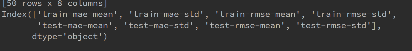
7. bst_cv是cv返回的结果，是一个DataFram的类型，其列为以下列组成

8.自定义评价函数：具体见这个博客：https://blog.csdn.net/wl_ss/article/details/78685984

 def customedscore(preds, dtrain):

     label = dtrain.get_label()

     pred = [int(i>=0.5) for i in preds]

     confusion_matrixs = confusion_matrix(label, pred)

     recall =float(confusion_matrixs[0][0]) / float(confusion_matrixs[0][1]+confusion_matrixs[0][0])

     precision = float(confusion_matrixs[0][0]) / float(confusion_matrixs[1][0]+confusion_matrixs[0][0])

     F = 5*precision* recall/(2*precision+3*recall)*100

     return 'FSCORE',float(F)

这种自定义的评价函数可以用于XGboost的cv函数或者train函数中的feval参数

还有一种定义评价函数的方式，如下

def mae_score(y_ture, y_pred):

    return mean_absolute_error(y_true=np.exp(y_ture), y_pred=np.exp(y_pred))

这种定义的函数可以用于gridSearchCV函数的scorning参数中。

xgboost调参步骤

第一步：确定n_estimators参数

首先初始化参数的值

xgb1 = XGBClassifier(max_depth=3,

                     learning_rate=0.1,

                     n_estimators=5000,

                     silent=False,

                     objective='binary:logistic',

                     booster='gbtree',

                     n_jobs=4,

                     gamma=0,

                     min_child_weight=1,

                     subsample=0.8,

                     colsample_bytree=0.8,

                     seed=7)

用cv函数求得参数n_estimators的最优值。

cv_result = xgb.cv(xgb1.get_xgb_params(),

                   dtrain,

                   num_boost_round=xgb1.get_xgb_params()['n_estimators'],

                   nfold=5,

                   metrics='auc',

                   early_stopping_rounds=50,

                   callbacks=[xgb.callback.early_stop(50),

                              xgb.callback.print_evaluation(period=1,show_stdv=True)])

第二步、确定max_depth和min_weight参数

param_grid = {'max_depth':[1,2,3,4,5],

             'min_child_weight':[1,2,3,4,5]}

grid_search = GridSearchCV(xgb1,param_grid,scoring='roc_auc',iid=False,cv=5)

grid_search.fit(train[feature_name],train['label'])

print('best_params:',grid_search.best_params_)

print('best_score:',grid_search.best_score_)

第三步、gamma参数调优

首先将上面调好的参数设置好，如下所示

xgb1 = XGBClassifier(max_depth=2,

                     learning_rate=0.1,

                     n_estimators=33,

                     silent=False,

                     objective='binary:logistic',

                     booster='gbtree',

                     n_jobs=4,

                     gamma=0,

                     min_child_weight=9,

                     subsample=0.8,

                     colsample_bytree=0.8,

                     seed=7)

然后继续网格调参

param_grid = {'gamma':[1,2,3,4,5,6,7,8,9]}

grid_search = GridSearchCV(xgb1,param_grid,scoring='roc_auc',iid=False,cv=5)

grid_search.fit(train[feature_name],train['label'])

print('best_params:',grid_search.best_params_)

print('best_score:',grid_search.best_score_)

第四步、调整subsample与colsample_bytree参数

param_grid = {'subsample':[i/10.0 for i in range(5,11)],

             'colsample_bytree':[i/10.0 for i in range(5,11)]}

grid_search = GridSearchCV(xgb1,param_grid,scoring='roc_auc',iid=False,cv=5)

grid_search.fit(train[feature_name],train['label'])

print('best_params:',grid_search.best_params_)

print('best_score:',grid_search.best_score_)

第五步、调整正则化参数

param_grid = {'reg_lambda':[i/10.0 for i in range(1,11)]}

grid_search = GridSearchCV(xgb1,param_grid,scoring='roc_auc',iid=False,cv=5)

grid_search.fit(train[feature_name],train['label'])

print('best_params:',grid_search.best_params_)

print('best_score:',grid_search.best_score_)

最后我们使用较低的学习率以及使用更多的决策树，可以用CV来实现这一步骤

xgb1 = XGBClassifier(max_depth=2,

                     learning_rate=0.01,

                     n_estimators=5000,

                     silent=False,

                     objective='binary:logistic',

                     booster='gbtree',

                     n_jobs=4,

                     gamma=2.1,

                     min_child_weight=9,

                     subsample=0.8,

                     colsample_bytree=0.8,

                     seed=7,

                     )

仅仅靠参数的调整和模型的小幅优化，想要让模型的表现有个大幅度提升是不可能的。
要想让模型的表现有一个质的飞跃，需要依靠其他的手段，诸如，特征工程(feature egineering) ，模型组合(ensemble of model),以及堆叠(stacking)等

具体的关于调参的知识请看以下链接：

https://www.cnblogs.com/TimVerion/p/11436001.html

http://www.pianshen.com/article/3311175716/