梯度下降法实现（Python语言描述）

原文地址：传送门

import numpy as np

import matplotlib.pyplot as plt

%matplotlib inline

plt.style.use(['ggplot'])

当你初次涉足机器学习时，你学习的第一个基本算法就是 梯度下降 (Gradient Descent), 可以说梯度下降法是机器学习算法的支柱。在这篇文章中，我尝试使用

python

python 解释梯度下降法的基本原理。一旦掌握了梯度下降法，很多问题就会变得容易理解，并且利于理解不同的算法。

如果你想尝试自己实现梯度下降法，你需要加载基本的

python

packages

packages ——

numpy

numpy and

matplotlib

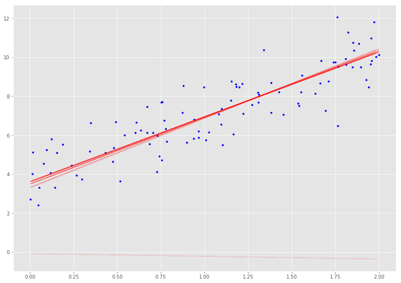
首先，我们将创建包含着噪声的线性数据

# 随机创建一些噪声

X = 2 * np.random.rand(100, 1)

y = 4 + 3 * X + np.random.randn(100, 1)

接下来通过 matplotlib 可视化数据

# 可视化数据

plt.plot(X, y, 'b.')

plt.xlabel("$x$", fontsize=18)

plt.ylabel("$y$", rotation=0, fontsize=18)

plt.axis([0, 2, 0, 15])

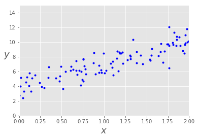
显然，

y 与

x 具有良好的线性关系，这个数据非常简单，只有一个自变量

我们可以将其表示为简单的线性关系：

y = b + mx

y=b+mx

并求出

b ,

m。

这种被称为解方程的分析方法并没有什么不妥，但机器学习是涉及矩阵计算的，因此我们使用矩阵法（向量法）进行分析。

我们将

y 替换成

(

)

J(\theta)

J(θ)，

b 替换成

\theta_0

θ0，

m 替换成

\theta_1

θ1。
得到如下表达式：

(

)

J(\theta) = \theta_0 + \theta_1 x

J(θ)=θ0+θ1x

注意： 本例中

\theta_0= 4

θ0=4，

\theta_1= 3

θ1=3

求解

\theta_0

θ0 和

\theta_1

θ1 的分析方法，代码如下：

X_b = np.c_[np.ones((100, 1)), X] # 为X添加了一个偏置单位，对于X中的每个向量都是1

theta_best = np.linalg.inv(X_b.T.dot(X_b)).dot(X_b.T).dot(y)

theta_best

array([[3.86687149],

       [3.12408839]])

不难发现这个值接近真实的

\theta_0

θ0，

\theta_1

θ1，由于我在数据中引入了噪声，所以存在误差。

X_new = np.array([[0], [2]])

X_new_b = np.c_[np.ones((2, 1)), X_new]

y_predict = X_new_b.dot(theta_best)

y_predict

array([[ 3.86687149],

       [10.11504826]])

梯度下降法（Gradient Descent）

Cost Function & Gradients

计算代价函数和梯度的公式如下所示。

注意：代价函数用于线性回归，对于其他算法，代价函数是不同的，梯度必须从代价函数中推导出来。

Cost

(

)

∑

(

)

(

)

−

(

)

J(\theta) = 1/2m \sum_{i=1}^{m} (h(\theta)^{(i)} - y^{(i)})^2

J(θ)=1/2mi=1∑m(h(θ)(i)−y(i))2

Gradient

∂

(

)

∂

∑

(

)

−

(

)

(

)

\frac{\partial J(\theta)}{\partial \theta_j} = 1/m\sum_{i=1}^{m}(h(\theta^{(i)} - y^{(i)}).X_j^{(i)}

∂θj∂J(θ)=1/mi=1∑m(h(θ(i)−y(i)).Xj(i)

Gradients

−

(

∑

(

)

−

(

)

(

)

\theta_0: = \theta_0 -\alpha . (1/m .\sum_{i=1}^{m}(h(\theta^{(i)} - y^{(i)}).X_0^{(i)})

θ0:=θ0−α.(1/m.i=1∑m(h(θ(i)−y(i)).X0(i))

−

(

∑

(

)

−

(

)

(

)

\theta_1: = \theta_1 -\alpha . (1/m .\sum_{i=1}^{m}(h(\theta^{(i)} - y^{(i)}).X_1^{(i)})

θ1:=θ1−α.(1/m.i=1∑m(h(θ(i)−y(i)).X1(i))

−

(

∑

(

)

−

(

)

(

)

\theta_2: = \theta_2 -\alpha . (1/m .\sum_{i=1}^{m}(h(\theta^{(i)} - y^{(i)}).X_2^{(i)})

θ2:=θ2−α.(1/m.i=1∑m(h(θ(i)−y(i)).X2(i))

−

(

∑

(

)

−

(

)

(

)

\theta_j: = \theta_j -\alpha . (1/m .\sum_{i=1}^{m}(h(\theta^{(i)} - y^{(i)}).X_0^{(i)})

θj:=θj−α.(1/m.i=1∑m(h(θ(i)−y(i)).X0(i))

def cal_cost(theta, X, y):

    '''

    Calculates the cost for given X and Y. The following shows and example of a single dimensional X

    theta = Vector of thetas

    X     = Row of X's np.zeros((2,j))

    y     = Actual y's np.zeros((2,1))

    where:

        j is the no of features

    '''

    m = len(y)

    predictions = X.dot(theta)

    cost = (1/2*m) * np.sum(np.square(predictions - y))

    return cost

def gradient_descent(X, y, theta, learning_rate = 0.01, iterations = 100):

    '''

    X    = Matrix of X with added bias units

    y    = Vector of Y

    theta=Vector of thetas np.random.randn(j,1)

    learning_rate

    iterations = no of iterations

    Returns the final theta vector and array of cost history over no of iterations

    '''

    m = len(y)

    # learning_rate = 0.01

    # iterations = 100

    cost_history = np.zeros(iterations)

    theta_history = np.zeros((iterations, 2))

    for i in range(iterations):

        prediction = np.dot(X, theta)

        theta = theta - (1/m) * learning_rate * (X.T.dot((prediction - y)))

        theta_history[i, :] = theta.T

        cost_history[i] = cal_cost(theta, X, y)

    return theta, cost_history, theta_history

# 从1000次迭代开始，学习率为0.01。从高斯分布的θ开始

lr =0.01

n_iter = 1000

theta = np.random.randn(2, 1)

X_b = np.c_[np.ones((len(X), 1)), X]

theta, cost_history, theta_history = gradient_descent(X_b, y, theta, lr, n_iter)

print('Theta0:          {:0.3f},\nTheta1:          {:0.3f}'.format(theta[0][0],theta[1][0]))

print('Final cost/MSE:  {:0.3f}'.format(cost_history[-1]))

Theta0:          3.867,

Theta1:          3.124

Final cost/MSE:  5457.747

# 绘制迭代的成本图

fig, ax = plt.subplots(figsize=(12,8))

ax.set_ylabel('J(Theta)')

ax.set_xlabel('Iterations')

ax.plot(range(1000), cost_history, 'b.')

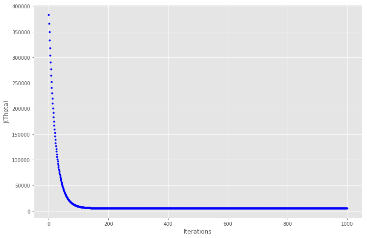
在大约 150 次迭代之后代价函数趋于稳定，因此放大到迭代200，看看曲线

fig, ax = plt.subplots(figsize=(10,8))

ax.plot(range(200), cost_history[:200], 'b.')

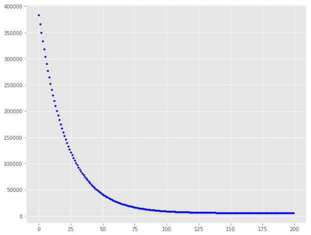
值得注意的是，最初成本下降得更快，然后成本降低的收益就不那么多了。我们可以尝试使用不同的学习速率和迭代组合，并得到不同学习率和迭代的效果会如何。

让我们建立一个函数，它可以显示效果，也可以显示梯度下降实际上是如何工作的。

def plot_GD(n_iter, lr, ax, ax1=None):

    '''

    n_iter = no of iterations

    lr = Learning Rate

    ax = Axis to plot the Gradient Descent

    ax1 = Axis to plot cost_history vs Iterations plot

    '''

    ax.plot(X, y, 'b.')

    theta = np.random.randn(2, 1)

    tr = 0.1

    cost_history = np.zeros(n_iter)

    for i in range(n_iter):

        pred_prev = X_b.dot(theta)

        theta, h, _ = gradient_descent(X_b, y, theta, lr, 1)

        pred = X_b.dot(theta)

        cost_history[i] = h[0]

        if ((i % 25 == 0)):

            ax.plot(X, pred, 'r-', alpha=tr)

            if tr < 0.8:

                tr += 0.2

    if not ax1 == None:

        ax1.plot(range(n_iter), cost_history, 'b.')

# 绘制不同迭代和学习率组合的图

fig = plt.figure(figsize=(30,25), dpi=200)

fig.subplots_adjust(hspace=0.4, wspace=0.4)

it_lr = [(2000, 0.001), (500, 0.01), (200, 0.05), (100, 0.1)]

count = 0

for n_iter, lr in it_lr:

    count += 1

    ax = fig.add_subplot(4, 2, count)

    count += 1

    ax1 = fig.add_subplot(4, 2, count)

    ax.set_title("lr:{}" .format(lr))

    ax1.set_title("Iterations:{}" .format(n_iter))

    plot_GD(n_iter, lr, ax, ax1)

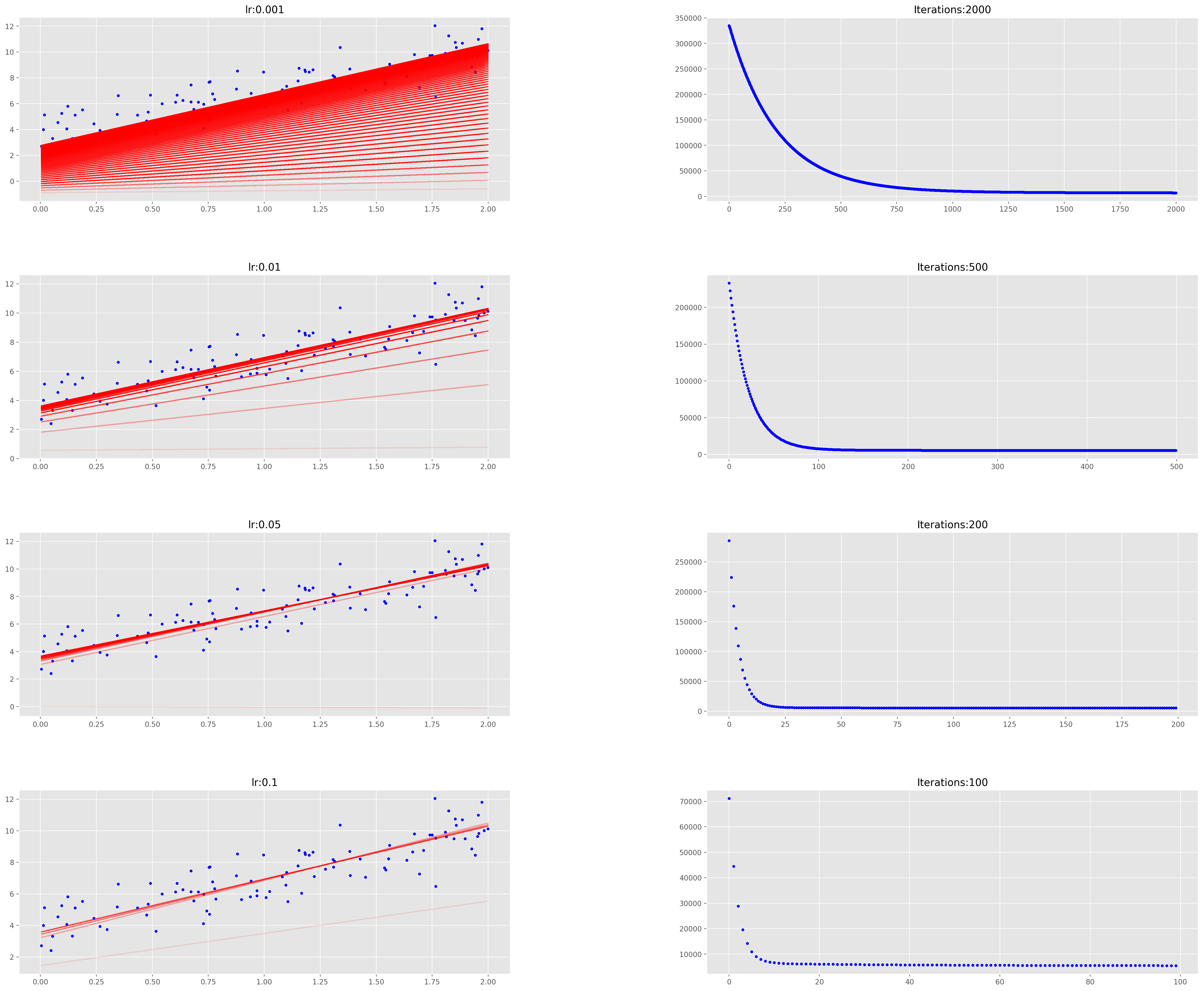
通过观察发现，以较小的学习速率收集解决方案需要很长时间，而学习速度越大，学习速度越快。

_, ax = plt.subplots(figsize=(14, 10))

plot_GD(100, 0.1, ax)

随机梯度下降法（Stochastic Gradient Descent）

随机梯度下降法，其实和批量梯度下降法原理类似，区别在与求梯度时没有用所有的

m 个样本的数据，而是仅仅选取一个样本

j 来求梯度。对应的更新公式是：

−

(

)

(

)

(

)

−

)

(

)

\theta_i = \theta_i - \alpha (h_\theta(x_0^{(j)}, x_1^{(j)}, ...x_n^{(j)}) - y_j)x_i^{(j)}

θi=θi−α(hθ(x0(j),x1(j),...xn(j))−yj)xi(j)

def stocashtic_gradient_descent(X, y, theta, learning_rate=0.01, iterations=10):

    '''

    X    = Matrix of X with added bias units

    y    = Vector of Y

    theta=Vector of thetas np.random.randn(j,1)

    learning_rate

    iterations = no of iterations

    Returns the final theta vector and array of cost history over no of iterations

    '''

    m = len(y)

    cost_history = np.zeros(iterations)

    for it in range(iterations):

        cost = 0.0

        for i in range(m):

            rand_ind = np.random.randint(0, m)

            X_i = X[rand_ind, :].reshape(1, X.shape[1])

            y_i = y[rand_ind, :].reshape(1, 1)

            prediction = np.dot(X_i, theta)

            theta -= (1/m) * learning_rate * (X_i.T.dot((prediction - y_i)))

            cost += cal_cost(theta, X_i, y_i)

        cost_history[it] = cost

    return theta, cost_history

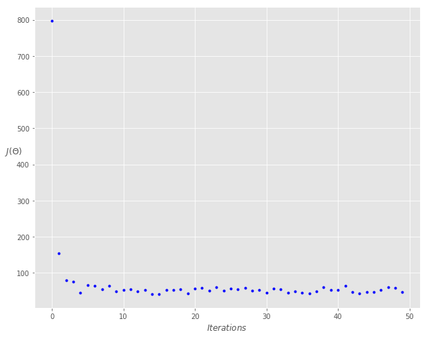
lr = 0.5

n_iter = 50

theta = np.random.randn(2,1)

X_b = np.c_[np.ones((len(X),1)), X]

theta, cost_history = stocashtic_gradient_descent(X_b, y, theta, lr, n_iter)

print('Theta0:          {:0.3f},\nTheta1:          {:0.3f}' .format(theta[0][0],theta[1][0]))

print('Final cost/MSE:  {:0.3f}' .format(cost_history[-1]))

Theta0:          3.762,

Theta1:          3.159

Final cost/MSE:  46.964

fig, ax = plt.subplots(figsize=(10,8))

ax.set_ylabel('$J(\Theta)$' ,rotation=0)

ax.set_xlabel('$Iterations$')

theta = np.random.randn(2,1)

ax.plot(range(n_iter), cost_history, 'b.')

小批量梯度下降法（Mini-batch Gradient Descent）

小批量梯度下降法是批量梯度下降法和随机梯度下降法的折衷，也就是对于

m 个样本，我们采用x个样子来迭代，

1<x<m

1<x<m。一般可以取

x=10

x=10，当然根据样本的数据，可以调整这个

x 的值。对应的更新公式是：

−

∑

−

(

)

(

)

(

)

−

)

(

)

\theta_i = \theta_i - \alpha \sum\limits_{j=t}^{t+x-1}(h_\theta(x_0^{(j)}, x_1^{(j)}, ...x_n^{(j)}) - y_j)x_i^{(j)}

θi=θi−αj=t∑t+x−1(hθ(x0(j),x1(j),...xn(j))−yj)xi(j)

def minibatch_gradient_descent(X, y, theta, learning_rate=0.01, iterations=10, batch_size=20):

    '''

    X    = Matrix of X without added bias units

    y    = Vector of Y

    theta=Vector of thetas np.random.randn(j,1)

    learning_rate

    iterations = no of iterations

    Returns the final theta vector and array of cost history over no of iterations

    '''

    m = len(y)

    cost_history = np.zeros(iterations)

    n_batches = int(m / batch_size)

    for it in range(iterations):

        cost = 0.0

        indices = np.random.permutation(m)

        X = X[indices]

        y = y[indices]

        for i in range(0, m, batch_size):

            X_i = X[i: i+batch_size]

            y_i = y[i: i+batch_size]

            X_i = np.c_[np.ones(len(X_i)), X_i]

            prediction = np.dot(X_i, theta)

            theta -= (1/m) * learning_rate * (X_i.T.dot((prediction - y_i)))

            cost += cal_cost(theta, X_i, y_i)

        cost_history[it] = cost

    return theta, cost_history

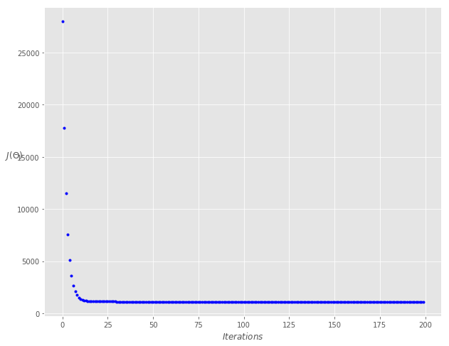
lr = 0.1

n_iter = 200

theta = np.random.randn(2, 1)

theta, cost_history = minibatch_gradient_descent(X, y, theta, lr, n_iter)

print('Theta0:          {:0.3f},\nTheta1:          {:0.3f}' .format(theta[0][0], theta[1][0]))

print('Final cost/MSE:  {:0.3f}' .format(cost_history[-1]))

Theta0:          3.842,

Theta1:          3.146

Final cost/MSE:  1090.518

fig, ax = plt.subplots(figsize=(10,8))

ax.set_ylabel('$J(\Theta)$', rotation=0)

ax.set_xlabel('$Iterations$')

theta = np.random.randn(2, 1)

ax.plot(range(n_iter), cost_history, 'b.')

参考：