sklearn——数据集调用及应用
忙了许久,总算是又想起这边还没写完呢。
那今天就写写sklearn库的一部分简单内容吧,包括数据集调用,聚类,轮廓系数等等。
自带数据集API
| 数据集函数 | 中文翻译 | 任务类型 | 数据规模 |
|---|---|---|---|
| load_boston | Boston房屋价格 | 回归 | 506*13 |
| fetch_california_housing | 加州住房 | 回归 | 20640*9 |
| load_diabetes | 糖尿病 | 回归 | 442*10 |
| load_digits | 手写字 | 分类 | 1797*64 |
| load_breast_cancer | 乳腺癌 | 分类、聚类 | (357+212)*30 |
| load_iris | 鸢尾花 | 分类、聚类 | (50*3)*4 |
| load_wine | 葡萄酒 | 分类 | (59+71+48)*13 |
| load_linnerud | 体能训练 | 多分类 | 20 |
提取信息关键字:
- DESCR:数据集的描述信息
- data:内部数据
- feature_names:数据字段名
- target:数据标签
- target_names:标签字段名(回归数据集无此项)
开始提取
以load_iris为例。
# 导入是必须的

from sklearn.datasets import load_iris

iris = load_iris()
iris # iris的所有信息,包括数据集、标签集、各字段名等
这个输出太长太乱,而且后边也有,我就不复制过来了
iris.keys() # 数据集关键字
dict_keys(['data', 'target', 'target_names', 'DESCR', 'feature_names'])
descr = iris['DESCR']

data = iris['data']

feature_names = iris['feature_names']

target = iris['target']

target_names = iris['target_names']
descr
'Iris Plants Database\n====================\n\nNotes\n-----\nData Set Characteristics:\n :Number of Instances: 150 (50 in each of three classes)\n :Number of Attributes: 4 numeric, predictive attributes and the class\n :Attribute Information:\n - sepal length in cm\n - sepal width in cm\n - petal length in cm\n - petal width in cm\n - class:\n - Iris-Setosa\n - Iris-Versicolour\n - Iris-Virginica\n :Summary Statistics:\n\n ============== ==== ==== ======= ===== ====================\n Min Max Mean SD Class Correlation\n ============== ==== ==== ======= ===== ====================\n sepal length: 4.3 7.9 5.84 0.83 0.7826\n sepal width: 2.0 4.4 3.05 0.43 -0.4194\n petal length: 1.0 6.9 3.76 1.76 0.9490 (high!)\n petal width: 0.1 2.5 1.20 0.76 0.9565 (high!)\n ============== ==== ==== ======= ===== ====================\n\n :Missing Attribute Values: None\n :Class Distribution: 33.3% for each of 3 classes.\n :Creator: R.A. Fisher\n :Donor: Michael Marshall (MARSHALL%PLU@io.arc.nasa.gov)\n :Date: July, 1988\n\nThis is a copy of UCI ML iris datasets.\nhttp://archive.ics.uci.edu/ml/datasets/Iris\n\nThe famous Iris database, first used by Sir R.A Fisher\n\nThis is perhaps the best known database to be found in the\npattern recognition literature. Fisher's paper is a classic in the field and\nis referenced frequently to this day. (See Duda & Hart, for example.) The\ndata set contains 3 classes of 50 instances each, where each class refers to a\ntype of iris plant. One class is linearly separable from the other 2; the\nlatter are NOT linearly separable from each other.\n\nReferences\n----------\n - Fisher,R.A. "The use of multiple measurements in taxonomic problems"\n Annual Eugenics, 7, Part II, 179-188 (1936); also in "Contributions to\n Mathematical Statistics" (John Wiley, NY, 1950).\n - Duda,R.O., & Hart,P.E. (1973) Pattern Classification and Scene Analysis.\n (Q327.D83) John Wiley & Sons. ISBN 0-471-22361-1. See page 218.\n - Dasarathy, B.V. (1980) "Nosing Around the Neighborhood: A New System\n Structure and Classification Rule for Recognition in Partially Exposed\n Environments". IEEE Transactions on Pattern Analysis and Machine\n Intelligence, Vol. PAMI-2, No. 1, 67-71.\n - Gates, G.W. (1972) "The Reduced Nearest Neighbor Rule". IEEE Transactions\n on Information Theory, May 1972, 431-433.\n - See also: 1988 MLC Proceedings, 54-64. Cheeseman et al"s AUTOCLASS II\n conceptual clustering system finds 3 classes in the data.\n - Many, many more ...\n'
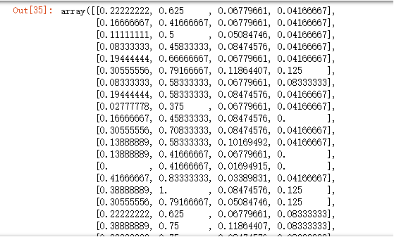
data
array([[5.1, 3.5, 1.4, 0.2],
[4.9, 3. , 1.4, 0.2],
[4.7, 3.2, 1.3, 0.2],
[4.6, 3.1, 1.5, 0.2],
[5. , 3.6, 1.4, 0.2],
[5.4, 3.9, 1.7, 0.4],
[4.6, 3.4, 1.4, 0.3],
[5. , 3.4, 1.5, 0.2],
[4.4, 2.9, 1.4, 0.2],
[4.9, 3.1, 1.5, 0.1],
[5.4, 3.7, 1.5, 0.2],
[4.8, 3.4, 1.6, 0.2],
[4.8, 3. , 1.4, 0.1],
[4.3, 3. , 1.1, 0.1],
[5.8, 4. , 1.2, 0.2],
[5.7, 4.4, 1.5, 0.4],
[5.4, 3.9, 1.3, 0.4],
[5.1, 3.5, 1.4, 0.3],
[5.7, 3.8, 1.7, 0.3],
[5.1, 3.8, 1.5, 0.3],
[5.4, 3.4, 1.7, 0.2],
[5.1, 3.7, 1.5, 0.4],
[4.6, 3.6, 1. , 0.2],
[5.1, 3.3, 1.7, 0.5],
[4.8, 3.4, 1.9, 0.2],
[5. , 3. , 1.6, 0.2],
[5. , 3.4, 1.6, 0.4],
[5.2, 3.5, 1.5, 0.2],
[5.2, 3.4, 1.4, 0.2],
[4.7, 3.2, 1.6, 0.2],
[4.8, 3.1, 1.6, 0.2],
[5.4, 3.4, 1.5, 0.4],
[5.2, 4.1, 1.5, 0.1],
[5.5, 4.2, 1.4, 0.2],
[4.9, 3.1, 1.5, 0.1],
[5. , 3.2, 1.2, 0.2],
[5.5, 3.5, 1.3, 0.2],
[4.9, 3.1, 1.5, 0.1],
[4.4, 3. , 1.3, 0.2],
[5.1, 3.4, 1.5, 0.2],
[5. , 3.5, 1.3, 0.3],
[4.5, 2.3, 1.3, 0.3],
[4.4, 3.2, 1.3, 0.2],
[5. , 3.5, 1.6, 0.6],
[5.1, 3.8, 1.9, 0.4],
[4.8, 3. , 1.4, 0.3],
[5.1, 3.8, 1.6, 0.2],
[4.6, 3.2, 1.4, 0.2],
[5.3, 3.7, 1.5, 0.2],
[5. , 3.3, 1.4, 0.2],
[7. , 3.2, 4.7, 1.4],
[6.4, 3.2, 4.5, 1.5],
[6.9, 3.1, 4.9, 1.5],
[5.5, 2.3, 4. , 1.3],
[6.5, 2.8, 4.6, 1.5],
[5.7, 2.8, 4.5, 1.3],
[6.3, 3.3, 4.7, 1.6],
[4.9, 2.4, 3.3, 1. ],
[6.6, 2.9, 4.6, 1.3],
[5.2, 2.7, 3.9, 1.4],
[5. , 2. , 3.5, 1. ],
[5.9, 3. , 4.2, 1.5],
[6. , 2.2, 4. , 1. ],
[6.1, 2.9, 4.7, 1.4],
[5.6, 2.9, 3.6, 1.3],
[6.7, 3.1, 4.4, 1.4],
[5.6, 3. , 4.5, 1.5],
[5.8, 2.7, 4.1, 1. ],
[6.2, 2.2, 4.5, 1.5],
[5.6, 2.5, 3.9, 1.1],
[5.9, 3.2, 4.8, 1.8],
[6.1, 2.8, 4. , 1.3],
[6.3, 2.5, 4.9, 1.5],
[6.1, 2.8, 4.7, 1.2],
[6.4, 2.9, 4.3, 1.3],
[6.6, 3. , 4.4, 1.4],
[6.8, 2.8, 4.8, 1.4],
[6.7, 3. , 5. , 1.7],
[6. , 2.9, 4.5, 1.5],
[5.7, 2.6, 3.5, 1. ],
[5.5, 2.4, 3.8, 1.1],
[5.5, 2.4, 3.7, 1. ],
[5.8, 2.7, 3.9, 1.2],
[6. , 2.7, 5.1, 1.6],
[5.4, 3. , 4.5, 1.5],
[6. , 3.4, 4.5, 1.6],
[6.7, 3.1, 4.7, 1.5],
[6.3, 2.3, 4.4, 1.3],
[5.6, 3. , 4.1, 1.3],
[5.5, 2.5, 4. , 1.3],
[5.5, 2.6, 4.4, 1.2],
[6.1, 3. , 4.6, 1.4],
[5.8, 2.6, 4. , 1.2],
[5. , 2.3, 3.3, 1. ],
[5.6, 2.7, 4.2, 1.3],
[5.7, 3. , 4.2, 1.2],
[5.7, 2.9, 4.2, 1.3],
[6.2, 2.9, 4.3, 1.3],
[5.1, 2.5, 3. , 1.1],
[5.7, 2.8, 4.1, 1.3],
[6.3, 3.3, 6. , 2.5],
[5.8, 2.7, 5.1, 1.9],
[7.1, 3. , 5.9, 2.1],
[6.3, 2.9, 5.6, 1.8],
[6.5, 3. , 5.8, 2.2],
[7.6, 3. , 6.6, 2.1],
[4.9, 2.5, 4.5, 1.7],
[7.3, 2.9, 6.3, 1.8],
[6.7, 2.5, 5.8, 1.8],
[7.2, 3.6, 6.1, 2.5],
[6.5, 3.2, 5.1, 2. ],
[6.4, 2.7, 5.3, 1.9],
[6.8, 3. , 5.5, 2.1],
[5.7, 2.5, 5. , 2. ],
[5.8, 2.8, 5.1, 2.4],
[6.4, 3.2, 5.3, 2.3],
[6.5, 3. , 5.5, 1.8],
[7.7, 3.8, 6.7, 2.2],
[7.7, 2.6, 6.9, 2.3],
[6. , 2.2, 5. , 1.5],
[6.9, 3.2, 5.7, 2.3],
[5.6, 2.8, 4.9, 2. ],
[7.7, 2.8, 6.7, 2. ],
[6.3, 2.7, 4.9, 1.8],
[6.7, 3.3, 5.7, 2.1],
[7.2, 3.2, 6. , 1.8],
[6.2, 2.8, 4.8, 1.8],
[6.1, 3. , 4.9, 1.8],
[6.4, 2.8, 5.6, 2.1],
[7.2, 3. , 5.8, 1.6],
[7.4, 2.8, 6.1, 1.9],
[7.9, 3.8, 6.4, 2. ],
[6.4, 2.8, 5.6, 2.2],
[6.3, 2.8, 5.1, 1.5],
[6.1, 2.6, 5.6, 1.4],
[7.7, 3. , 6.1, 2.3],
[6.3, 3.4, 5.6, 2.4],
[6.4, 3.1, 5.5, 1.8],
[6. , 3. , 4.8, 1.8],
[6.9, 3.1, 5.4, 2.1],
[6.7, 3.1, 5.6, 2.4],
[6.9, 3.1, 5.1, 2.3],
[5.8, 2.7, 5.1, 1.9],
[6.8, 3.2, 5.9, 2.3],
[6.7, 3.3, 5.7, 2.5],
[6.7, 3. , 5.2, 2.3],
[6.3, 2.5, 5. , 1.9],
[6.5, 3. , 5.2, 2. ],
[6.2, 3.4, 5.4, 2.3],
[5.9, 3. , 5.1, 1.8]])
feature_names
['sepal length (cm)',
'sepal width (cm)',
'petal length (cm)',
'petal width (cm)']
target
array([0, 0, 0, 0, 0, 0, 0, 0, 0, 0, 0, 0, 0, 0, 0, 0, 0, 0, 0, 0, 0, 0,
0, 0, 0, 0, 0, 0, 0, 0, 0, 0, 0, 0, 0, 0, 0, 0, 0, 0, 0, 0, 0, 0,
0, 0, 0, 0, 0, 0, 1, 1, 1, 1, 1, 1, 1, 1, 1, 1, 1, 1, 1, 1, 1, 1,
1, 1, 1, 1, 1, 1, 1, 1, 1, 1, 1, 1, 1, 1, 1, 1, 1, 1, 1, 1, 1, 1,
1, 1, 1, 1, 1, 1, 1, 1, 1, 1, 1, 1, 2, 2, 2, 2, 2, 2, 2, 2, 2, 2,
2, 2, 2, 2, 2, 2, 2, 2, 2, 2, 2, 2, 2, 2, 2, 2, 2, 2, 2, 2, 2, 2,
2, 2, 2, 2, 2, 2, 2, 2, 2, 2, 2, 2, 2, 2, 2, 2, 2, 2])
target_names
array(['setosa', 'versicolor', 'virginica'], dtype='<U10')
小试一下
from sklearn.cluster import KMeans  # 聚类包

from sklearn.preprocessing import StandardScaler, MinMaxScaler  # 预处理包
# 标准差标准化

# 公式:(x-mean(X))/std(X)

scale = StandarScaler().fit(data)  # 训练规则

X = scale.transform(data)  # 应用规则
# 离差标准化(零一标准化)

# 公式:(x-min(X))/(max(X)-min(X))

scale = MinMaxScaler().fit(data)  # 训练规则

X = scale.transform(data)  # 应用规则

X
clf = KMeans(n_clusters = 3, random_state = 123).fit(X) # 聚成3类
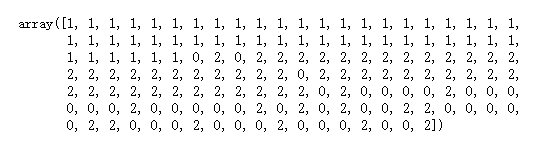
clf.labels_
kmeans = KMeans(n_clusters = 3, random_state = 123).fit(data) # 用data对比一下
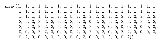
kmeans.labels_
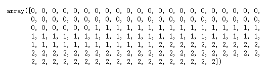
target # 这里我们也可以再拿出原始标签相互对比
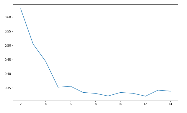
当然啦,先人们也是一早就想着:得找个办法来衡量一下聚类效果啊。
于是乎,轮廓系数就诞生了。
且看下方代码。
'''这里插入一下轮廓系数的一些知识点吧

1.对于第i个对象,计算它到所属簇中所有其他对象的平均距离,记ai(体现凝聚度)

2.对于第i个对象和不包含该对象的任意簇,计算该对象到给定簇中所有对象的平均距离,取最小,记bi(体现分离度)

3.第i个对象的轮廓系数为si=(bi-ai)/max(ai, bi)

	所以,很明显:轮廓系数取值为[-1,1],且越大越好;若值为负,即ai>bi,说明样本被分配到错误的簇中,不可接受;若值接近0,ai≈bi,表明聚类结果有重叠的情况。

'''

from sklearn.metrics import silhouette_score  # 轮廓系数

import matplotlib.pyplot as plt

silhouettteScore = []

for i in range(2,15):

    kmeans = KMeans(n_clusters = i,random_state=123).fit(X) ##构建并训练模型

    score = silhouette_score(X,kmeans.labels_)  # X是零一化之后的数据

    silhouettteScore.append(score)

plt.figure(figsize=(10,6))

plt.plot(range(2,15),silhouettteScore,linewidth=1.5, linestyle="-")

plt.show()
嗯,到此先结束吧,等下一篇我们再继续讲构建回归模型。
sklearn——数据集调用及应用的更多相关文章
- sklearn中调用PCA算法
sklearn中调用PCA算法 PCA算法是一种数据降维的方法,它可以对于数据进行维度降低,实现提高数据计算和训练的效率,而不丢失数据的重要信息,其sklearn中调用PCA算法的具体操作和代码如下所 ...
- 【学习笔记】sklearn数据集与估计器
数据集划分 机器学习一般的数据集会划分为两个部分: 训练数据:用于训练,构建模型 测试数据:在模型检验时使用,用于评估模型是否有效 训练数据和测试数据常用的比例一般为:70%: 30%, 80%: 2 ...
- Sklearn数据集与机器学习
sklearn数据集与机器学习组成 机器学习组成:模型.策略.优化 <统计机器学习>中指出:机器学习=模型+策略+算法.其实机器学习可以表示为:Learning= Representati ...
- 机器学习笔记(四)--sklearn数据集
sklearn数据集 (一)机器学习的一般数据集会划分为两个部分 训练数据:用于训练,构建模型. 测试数据:在模型检验时使用,用于评估模型是否有效. 划分数据的API:sklearn.model_se ...
- sklearn数据集
数据集划分: 机器学习一般的数据集会划分为两个部分 训练数据: 用于训练,构建模型 测试数据: 在模型检验时使用,用于评估模型是否有效 sklearn数据集划分API: 代码示例文末! scikit- ...
- sklearn数据集划分
sklearn数据集划分方法有如下方法: KFold,GroupKFold,StratifiedKFold,LeaveOneGroupOut,LeavePGroupsOut,LeaveOneOut,L ...
- sklearn中调用集成学习算法
1.集成学习是指对于同一个基础数据集使用不同的机器学习算法进行训练,最后结合不同的算法给出的意见进行决策,这个方法兼顾了许多算法的"意见",比较全面,因此在机器学习领域也使用地非常 ...
- SKLearn数据集API(一)
注:本文是人工智能研究网的学习笔记 数据集一览 类型 获取方式 自带的小数据集 sklearn.datasets.load_ 在线下载的数据集 sklearn.datasets.fetch_ 计算机生 ...
- SKLearn数据集API(二)
注:本文是人工智能研究网的学习笔记 计算机生成的数据集 用于分类任务和聚类任务,这些函数产生样本特征向量矩阵以及对应的类别标签集合. 数据集 简介 make_blobs 多类单标签数据集,为每个类分配 ...
随机推荐
- nodejs结合apiblue实现MockServer
apiblue功能很强大,里面支持很多插件,这些插件能够为restfulAPI提供接口文档自动生成,甚至Mockserver的功能,当然,好多插件还是有很多坑的.下面用apiblue实现下面的业务需求 ...
- Selenium自动化测试Python四:WebDriver封装
WebDriver 封装 欢迎阅读WebDriver封装讲义.本篇讲义将会重点介绍Selenium WebDriver API的封装的概念和方法,以及使用封装进行自动化测试的设计. WebDriver ...
- KahaDB简介
ActiveMQ 5.3以后,出现了KahaDB.她是一个基于文件支持事务的消息存储器,是一个可靠,高性能,可扩展的消息存储器. 她的设计初衷就是使用简单并尽可能的快.KahaDB的索引使用一 ...
- 分享一套简单的CodeSmith三层模板
如果要连接mysql,需要安装驱动: https://cdn.mysql.com//Downloads/Connector-Net/mysql-connector-net-8.0.12.msi 连接字 ...
- 微信小程序图片变形解决方法
微信小程序的image标签中有个mode属性,使用aspectFill即可 注:image组件默认宽度300px.高度225px mode 有效值: mode 有 13 种模式,其中 4 种是缩放模式 ...
- Tomcat8源码编译及导入Eclipse中研究
最近因为需求需要修改Tomcat中的某些功能,无奈只能研究那部分源码然后稍作修改. 目前Tomcat最新版是8.0,下载了源码包,编译并导入Eclipse中研究比较方便. 1. Tomcat8源码编译 ...
- ElasticSearch 基础<转载>
使用curl命令操作elasticsearch 大岩不灿 发表于 2015年4月25日 浏览 13,463 次 第一:_cat系列_cat系列提供了一系列查询elasticsearch集群状态的接口. ...
- WebMagic之爬虫监控
访问我的博客 前言 年前闲着无聊,研究了一阵子爬虫技术,接触到爬虫框架 WebMagic,感觉很好用. 在之后的工作中,接手了新站与第三方接口对接的工作,主要的工作是去抓取对方接口的内容:初始的时候, ...
- 利用docker hub做中转拉取google的k8s镜像
1.背景 部署kubernetes,需要FQ.但是在初始化的时候,即是FQ了有的镜像pull依然会超时,导致初始化失败.而你又不想使用国内的一些镜像源,因为更新不及时.很多新功能和插件都不会包括,只想 ...
- 【WePY小程序框架实战三】-组件传值
[WePY小程序框架实战一]-创建项目 [WePY小程序框架实战二]-页面结构 父子组件传值 静态传值 静态传值为父组件向子组件传递常量数据,因此只能传递String字符串类型. 父组件 (paren ...