(转) Learning from Imbalanced Classes

Learning from Imbalanced Classes

AUGUST 25TH, 2016

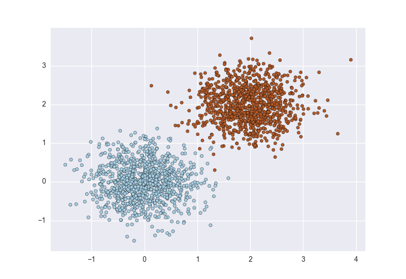
If you’re fresh from a machine learning course, chances are most of the datasets you used were fairly easy. Among other things, when you built classifiers, the example classes werebalanced, meaning there were approximately the same number of examples of each class. Instructors usually employ cleaned up datasets so as to concentrate on teaching specific algorithms or techniques without getting distracted by other issues. Usually you’re shown examples like the figure below in two dimensions, with points representing examples and different colors (or shapes) of the points representing the class:

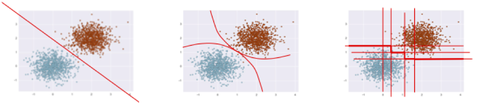
The goal of a classification algorithm is to attempt to learn a separator (classifier) that can distinguish the two. There are many ways of doing this, based on various mathematical, statistical, or geometric assumptions:

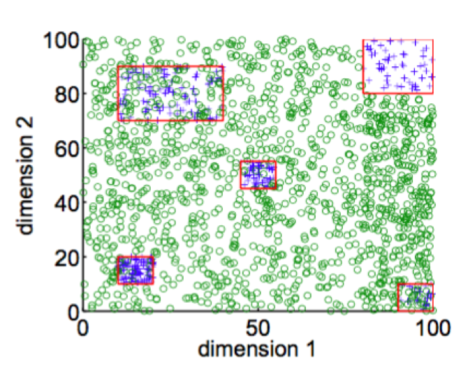
But when you start looking at real, uncleaned data one of the first things you notice is that it’s a lot noisier and imbalanced. Scatterplots of real data often look more like this:

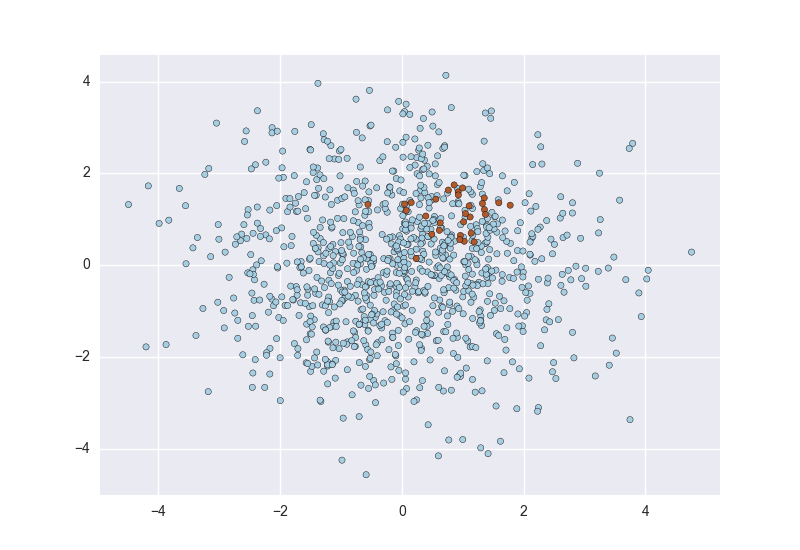
The primary problem is that these classes are imbalanced: the red points are greatly outnumbered by the blue.

Research on imbalanced classes often considers imbalanced to mean a minority class of 10% to 20%. In reality, datasets can get far more imbalanced than this. —Here are some examples:

1. About 2% of credit card accounts are defrauded per year1. (Most fraud detection domains are heavily imbalanced.)
2. Medical screening for a condition is usually performed on a large population of people without the condition, to detect a small minority with it (e.g., HIV prevalence in the USA is ~0.4%).
3. Disk drive failures are approximately ~1% per year.
4. The conversion rates of online ads has been estimated to lie between 10-3 to 10-6.
5. Factory production defect rates typically run about 0.1%.

Many of these domains are imbalanced because they are what I call needle in a haystackproblems, where machine learning classifiers are used to sort through huge populations of negative (uninteresting) cases to find the small number of positive (interesting, alarm-worthy) cases.

When you encounter such problems, you’re bound to have difficulties solving them with standard algorithms. Conventional algorithms are often biased towards the majority class because their loss functions attempt to optimize quantities such as error rate, not taking the data distribution into consideration2. In the worst case, minority examples are treated as outliers of the majority class and ignored. The learning algorithm simply generates a trivial classifier that classifies every example as the majority class.

This might seem like pathological behavior but it really isn’t. Indeed, if your goal is to maximize simple accuracy (or, equivalently, minimize error rate), this is a perfectly acceptable solution. But if we assume that the rare class examples are much more important to classify, then we have to be more careful and more sophisticated about attacking the problem.

If you deal with such problems and want practical advice on how to address them, read on.

Note: The point of this blog post is to give insight and concrete advice on how to tackle such problems. However, this is not a coding tutorial that takes you line by line through code. I have Jupyter Notebooks (also linked at the end of the post) useful for experimenting with these ideas, but this blog post will explain some of the fundamental ideas and principles.

Handling imbalanced data

Learning from imbalanced data has been studied actively for about two decades in machine learning. It’s been the subject of many papers, workshops, special sessions, and dissertations (a recent survey has about 220 references). A vast number of techniques have been tried, with varying results and few clear answers. Data scientists facing this problem for the first time often ask What should I do when my data is imbalanced? This has no definite answer for the same reason that the general question Which learning algorithm is best? has no definite answer: it depends on the data.

That said, here is a rough outline of useful approaches. These are listed approximately in order of effort:

• Do nothing. Sometimes you get lucky and nothing needs to be done. You can train on the so-called natural (or stratified) distribution and sometimes it works without need for modification.
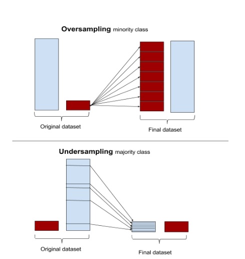
• Balance the training set in some way:
  • Oversample the minority class.
  • Undersample the majority class.
  • Synthesize new minority classes.
• Throw away minority examples and switch to an anomaly detection framework.
• At the algorithm level, or after it:
  • Adjust the class weight (misclassification costs).
  • Adjust the decision threshold.
  • Modify an existing algorithm to be more sensitive to rare classes.
• Construct an entirely new algorithm to perform well on imbalanced data.

Digression: evaluation dos and don’ts

First, a quick detour. Before talking about how to train a classifier well with imbalanced data, we have to discuss how to evaluate one properly. This cannot be overemphasized. You can only make progress if you’re measuring the right thing.

1. Don’t use accuracy (or error rate) to evaluate your classifier! There are two significant problems with it. Accuracy applies a naive 0.50 threshold to decide between classes, and this is usually wrong when the classes are imbalanced. Second, classification accuracy is based on a simple count of the errors, and you should know more than this. You should know which classes are being confused and where (top end of scores, bottom end, throughout?). If you don’t understand these points, it might be helpful to read The Basics of Classifier Evaluation, Part 2. You should be visualizing classifier performance using a ROC curve, a precision-recall curve, a lift curve, or a profit (gain) curve.
   

   ROC curve

   

   Precision-recall curve

2. Don’t get hard classifications (labels) from your classifier (via score3 or predict). Instead, get probability estimates via proba or predict_proba.
3. When you get probability estimates, don’t blindly use a 0.50 decision threshold to separate classes. Look at performance curves and decide for yourself what threshold to use (see next section for more on this). Many errors were made in early papers because researchers naively used 0.5 as a cut-off.
4. No matter what you do for training, always test on the natural (stratified) distribution your classifier is going to operate upon. Seesklearn.cross_validation.StratifiedKFold.
5. You can get by without probability estimates, but if you need them, use calibration (seesklearn.calibration.CalibratedClassifierCV)

The two-dimensional graphs in the first bullet above are always more informative than a single number, but if you need a single-number metric, one of these is preferable to accuracy:

1. The Area Under the ROC curve (AUC) is a good general statistic. It is equal to the probability that a random positive example will be ranked above a random negative example.
2. The F1 Score is the harmonic mean of precision and recall. It is commonly used in text processing when an aggregate measure is sought.
3. Cohen’s Kappa is an evaluation statistic that takes into account how much agreement would be expected by chance.

Oversampling and undersampling

The easiest approaches require little change to the processing steps, and simply involve adjusting the example sets until they are balanced. Oversampling randomly replicates minority instances to increase their population. Undersampling randomly downsamples the majority class. Some data scientists (naively) think that oversampling is superior because it results in more data, whereas undersampling throws away data. But keep in mind that replicating data is not without consequence—since it results in duplicate data, it makes variables appear to have lower variance than they do. The positive consequence is that it duplicates the number of errors: if a classifier makes a false negative error on the original minority data set, and that data set is replicated five times, the classifier will make six errors on the new set. Conversely, undersampling can make the independent variables look like they have a higher variance than they do.

Because of all this, the machine learning literature shows mixed results with oversampling, undersampling, and using the natural distributions.

Most machine learning packages can perform simple sampling adjustment. The R packageunbalanced implements a number of sampling techniques specific to imbalanced datasets, and scikit-learn.cross_validation has basic sampling algorithms.

Bayesian argument of Wallace et al.

Possibly the best theoretical argument of—and practical advice for—class imbalance was put forth in the paper Class Imbalance, Redux, by Wallace, Small, Brodley and Trikalinos4. They argue for undersampling the majority class. Their argument is mathematical and thorough, but here I’ll only present an example they use to make their point.

They argue that two classes must be distinguishable in the tail of some distribution of some explanatory variable. Assume you have two classes with a single dependent variable, x. Each class is generated by a Gaussian with a standard deviation of 1. The mean of class 1 is 1 and the mean of class 2 is 2. We shall arbitrarily call class 2 the majority class. They look like this:

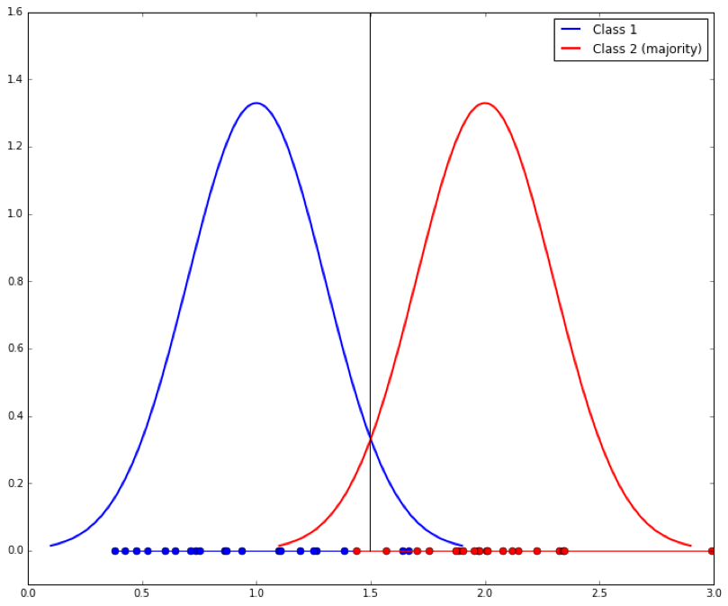
Given an x value, what threshold would you use to determine which class it came from? It should be clear that the best separation line between the two is at their midpoint, x=1.5, shown as the vertical line: if a new example x falls under 1.5 it is probably Class 1, else it is Class 2. When learning from examples, we would hope that a discrimination cutoff at 1.5 is what we would get, and if the classes are evenly balanced this is approximately what we should get. The dots on the x axis show the samples generated from each distribution.

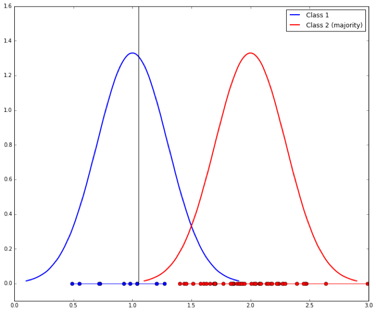
But we’ve said that Class 1 is the minority class, so assume that we have 10 samples from it and 50 samples from Class 2. It is likely we will learn a shifted separation line, like this:

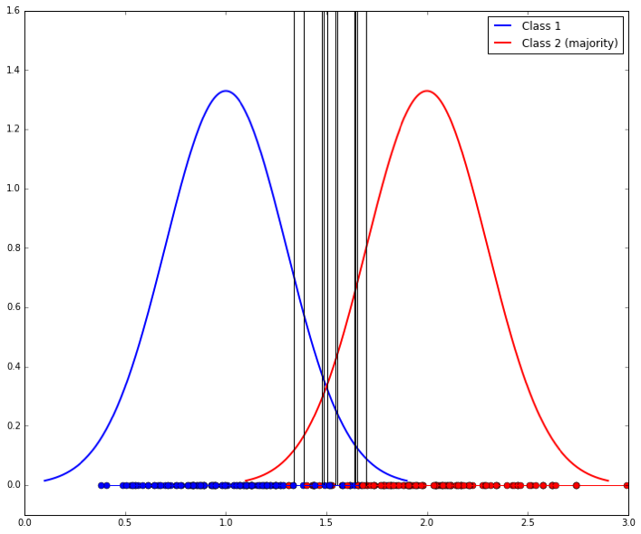
We can do better by down-sampling the majority class to match that of the minority class. The problem is that the separating lines we learn will have high variability (because the samples are smaller), as shown here (ten samples are shown, resulting in ten vertical lines):

So a final step is to use bagging to combine these classifiers. The entire process looks like this:

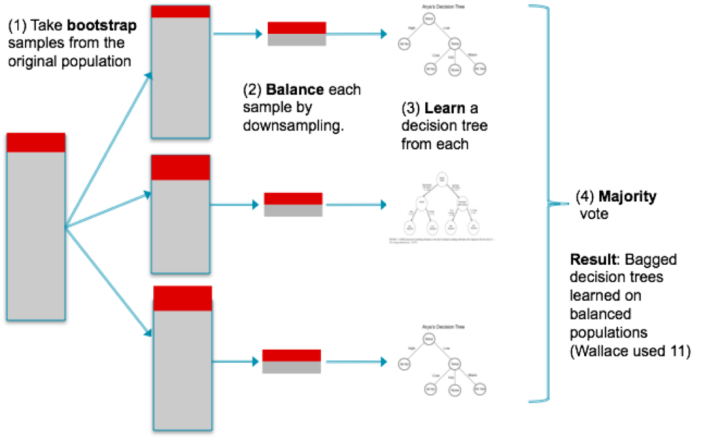
This technique has not been implemented in Scikit-learn, though a file called blagging.py(balanced bagging) is available that implements a BlaggingClassifier, which balances bootstrapped samples prior to aggregation.

Neighbor-based approaches

Over- and undersampling selects examples randomly to adjust their proportions. Other approaches examine the instance space carefully and decide what to do based on their neighborhoods.

For example, Tomek links are pairs of instances of opposite classes who are their own nearest neighbors. In other words, they are pairs of opposing instances that are very close together.

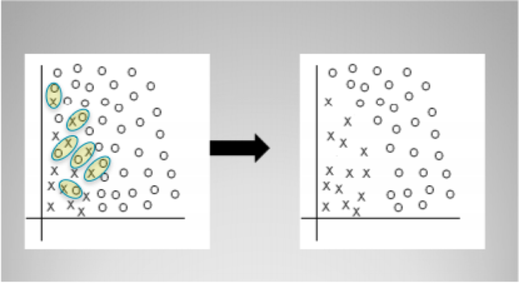
Tomek’s algorithm looks for such pairs and removes the majority instance of the pair. The idea is to clarify the border between the minority and majority classes, making the minority region(s) more distinct. The diagram above shows a simple example of Tomek link removal. The R package unbalanced implements Tomek link removal, as does a number of sampling techniques specific to imbalanced datasets. Scikit-learn has no built-in modules for doing this, though there are some independent packages (e.g., TomekLink).

Synthesizing new examples: SMOTE and descendants

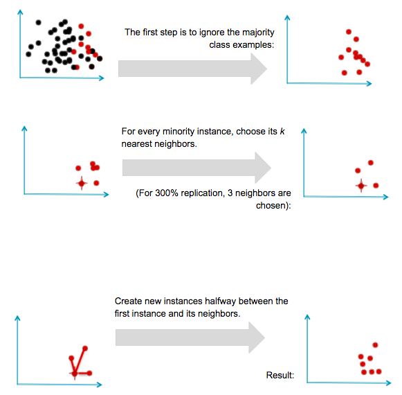
Another direction of research has involved not resampling of examples, but synthesis of new ones. The best known example of this approach is Chawla’s SMOTE (Synthetic Minority Oversampling TEchnique) system. The idea is to create new minority examples by interpolating between existing ones. The process is basically as follows. Assume we have a set of majority and minority examples, as before:

SMOTE was generally successful and led to many variants, extensions, and adaptations to different concept learning algorithms. SMOTE and variants are available in R in theunbalanced package and in Python in the UnbalancedDataset package.

It is important to note a substantial limitation of SMOTE. Because it operates by interpolating between rare examples, it can only generate examples within the body of available examples—never outside. Formally, SMOTE can only fill in the convex hull of existing minority examples, but not create new exterior regions of minority examples.

Adjusting class weights

Many machine learning toolkits have ways to adjust the “importance” of classes. Scikit-learn, for example, has many classifiers that take an optional class_weight parameter that can be set higher than one. Here is an example, taken straight from the scikit-learn documentation, showing the effect of increasing the minority class’s weight by ten. The solid black line shows the separating border when using the default settings (both classes weighed equally), and the dashed line after the class_weight parameter for the minority (red) classes changed to ten.

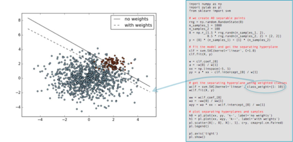
As you can see, the minority class gains in importance (its errors are considered more costly than those of the other class) and the separating hyperplane is adjusted to reduce the loss.

It should be noted that adjusting class importance usually only has an effect on the cost of class errors (False Negatives, if the minority class is positive). It will adjust a separating surface to decrease these accordingly. Of course, if the classifier makes no errors on the training set errors then no adjustment may occur, so altering class weights may have no effect.

And beyond

This post has concentrated on relatively simple, accessible ways to learn classifiers from imbalanced data. Most of them involve adjusting data before or after applying standard learning algorithms. It’s worth briefly mentioning some other approaches.

New algorithms

Learning from imbalanced classes continues to be an ongoing area of research in machine learning with new algorithms introduced every year. Before concluding I’ll mention a few recent algorithmic advances that are promising.

In 2014 Goh and Rudin published a paper Box Drawings for Learning with Imbalanced Data5which introduced two algorithms for learning from data with skewed examples. These algorithms attempt to construct “boxes” (actually axis-parallel hyper-rectangles) around clusters of minority class examples:

Their goal is to develop a concise, intelligible representation of the minority class. Their equations penalize the number of boxes and the penalties serve as a form of regularization.

They introduce two algorithms, one of which (Exact Boxes) uses mixed-integer programming to provide an exact but fairly expensive solution; the other (Fast Boxes) uses a faster clustering method to generate the initial boxes, which are subsequently refined. Experimental results show that both algorithms perform very well among a large set of test datasets.

Earlier I mentioned that one approach to solving the imbalance problem is to discard the minority examples and treat it as a single-class (or anomaly detection) problem. One recent anomaly detection technique has worked surprisingly well for just that purpose. Liu, Ting and Zhou introduced a technique called Isolation Forests6 that attempted to identify anomalies in data by learning random forests and then measuring the average number of decision splits required to isolate each particular data point. The resulting number can be used to calculate each data point’s anomaly score, which can also be interpreted as the likelihood that the example belongs to the minority class. Indeed, the authors tested their system using highly imbalanced data and reported very good results. A follow-up paper by Bandaragoda, Ting, Albrecht, Liu and Wells7 introduced Nearest Neighbor Ensembles as a similar idea that was able to overcome several shortcomings of Isolation Forests.

Buying or creating more data

As a final note, this blog post has focused on situations of imbalanced classes under the tacit assumption that you’ve been given imbalanced data and you just have to tackle the imbalance. In some cases, as in a Kaggle competition, you’re given a fixed set of data and you can’t ask for more.

But you may face a related, harder problem: you simply don’t have enough examples of the rare class. None of the techniques above are likely to work. What do you do?

In some real world domains you may be able to buy or construct examples of the rare class. This is an area of ongoing research in machine learning. If rare data simply needs to be labeled reliably by people, a common approach is to crowdsource it via a service likeMechanical Turk. Reliability of human labels may be an issue, but work has been done in machine learning to combine human labels to optimize reliability. Finally, Claudia Perlich in her Strata talk All The Data and Still Not Enough gives examples of how problems with rare or non-existent data can be finessed by using surrogate variables or problems, essentially using proxies and latent variables to make seemingly impossible problems possible. Related to this is the strategy of using transfer learning to learn one problem and transfer the results to another problem with rare examples, as described here.

Comments or questions?

Here, I have attempted to distill most of my practical knowledge into a single post. I know it was a lot, and I would value your feedback. Did I miss anything important? Any comments or questions on this blog post are welcome.

Resources and further reading

1. Several Jupyter notebooks are available illustrating aspects of imbalanced learning.
   • A notebook illustrating sampled Gaussians, above, is at Gaussians.ipynb.
   • A simple implementation of Wallace’s method is available at blagging.py. It is a simple fork of the existing bagging implementation of sklearn, specifically./sklearn/ensemble/bagging.py.
   • A notebook using this method is available at ImbalancedClasses.ipynb. It loads up several domains and compares blagging with other methods under different distributions.
2. Source code for Box Drawings in MATLAB is available from:http://web.mit.edu/rudin/www/code/BoxDrawingsCode.zip
3. Source code for Isolation Forests in R is available at:https://sourceforge.net/projects/iforest/

Thanks to Chloe Mawer for her Jupyter Notebook design work.

1. Natalie Hockham makes this point in her talk Machine learning with imbalanced data sets, which focuses on imbalance in the context of credit card fraud detection.
2. By definition there are fewer instances of the rare class, but the problem comes about because the cost of missing them (a false negative) is much higher.
3. The details in courier are specific to Python’s Scikit-learn.
4. “Class Imbalance, Redux”. Wallace, Small, Brodley and Trikalinos. IEEE Conf on Data Mining. 2011.
5. Box Drawings for Learning with Imbalanced Data.” Siong Thye Goh and Cynthia Rudin. KDD-2014, August 24–27, 2014, New York, NY, USA.
6. “Isolation-Based Anomaly Detection”. Liu, Ting and Zhou. ACM Transactions on Knowledge Discovery from Data, Vol. 6, No. 1. 2012.
7. “Efficient Anomaly Detection by Isolation Using Nearest Neighbour Ensemble.” Bandaragoda, Ting, Albrecht, Liu and Wells. ICDM-2014