Graphical Analysis of German Parliament Voting Pattern

We use network visualizations to look into the voting patterns in the current German parliament. I downloaded the data here and all figures can be reproduced using the R code available on Github.

Missing values, invalid votes, abstention from voting and not showing up for the vote weres coded as (-1), such that all other responses are a yes (1) or no (2) vote. We use pearson correlation as a measure of voting similarity and voting behavior coded as (-1) is regarded as noise in the dataset. 36 of the 659 members of parliament were removed from the data because more than 50% of the votes were coded as (-1). The reason was that they either joined or left the parliament during the analyzed time period.

Disclaimer: note that only for a fraction of the bills passed in the German parliament votes are recorded (and used here) and that relations between single members of parliaments might be artifacts of the noise-coding. Moreover, the data is quite scarce (136 bills). Therefore we should not draw any strong conclusions from this coarse-grained analysis.

Voting Pattern Amongst Members of Parliament

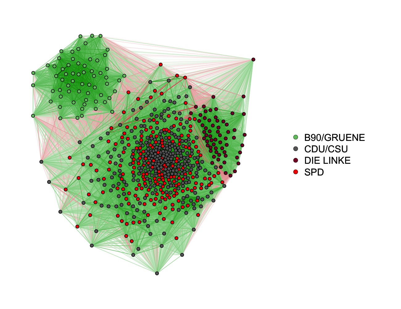
We first compute the correlations between the voting behavior of all pairs of members of parliament, which gives us a 623 x 623 correlation matrix. We then visualize this correlation matrix using the force-directed Fruchterman Reingold algorithm as implemented in the qgraph package. This algorithm puts nodes (politicians) on the plane such that edges (connections) have comparable length and that edges are crossing as little as possible.

(For readers on R-Bloggers.com: click here for the original post with larger figures.)

Green edges indicate positive correlations (voter agreement) and red edges indicate negative correlations (voter disagreement). The width of the edges is proportional to the strength (absolute value) of the correlation. We see that the green party (B90/GRUENE) clusters together, as well as the left party (DIE LINKE). The third and biggest cluster consists of members of the two largest parties, the social democrats (SPD) and the conservatives (CDU/CSU). This is the structure we would expect intuitively, as social democrats and conservatives currently form the government in a grand coalition.

With some imagination, one could also identify a couple of subclusters in this large cluster. A detailed analysis of smaller clusters would be especially interesting if we had additional information about politicians. We could then see whether the cluster assignment computed from the voting behavior relates to these additional variables. For instance, politicians with close ties to the economy might vote together, irrespective of their party.

So far we assumed that we can adequately describe the voting pattern of the whole period from 26.11.2013 - 14.04.2016 with one graph. This implies that we assume that the relative voting behavior does not change over time. For example, this means that if members of parliament A and B agree on votes at the beginning of the period, they also agree throughout the rest of the period and do not start to disagree at some point. In the next section we check whether the voting behavior changes over time.

Voting Pattern Amongst Members of Parliament across Time

To make graphs comparable over different time points and to be able to see growing (dis-) agreement between parties, we arrange individual members of parliament in circles that correspond to their parties. We compute a time-varying graph by visualizing a Gaussian kernel smoothed (bandwidth = .1, time interval [0,1]) correlation matrix at 20 equally spaced time points. Details can be found in the code used to create all figures, which is available here. We then combine these 20 graphs into the following video:

We see that right after the time the parliament was elected and the big coalition was formed in November 2013, there is relatively high agreement between members of CDU/CSU and SPD. Within the next three years, however, the agreement decreasees. With regards to the parties in the opposition, at the beginning of the period the green and the left party disagree to a similar degree with the grand coalition. Over time, however, it appears that the green party increasingly agrees with the grand coalition, while the left party agrees less and less with the CDU/CSU- and SPD-led government.

As the number of seats the parties have in the parliament differs widely, it is hard to read agreement within parties from the above graph. For instance, the cycle of CDU/CSU seems to be filled with more and thicker green edges than the one of SPD, however, this could well be because there are simply more politicians (307 vs. 191) and hence more edges displayed. Therefore, we have a closer look at within-party agreement in the following graph:

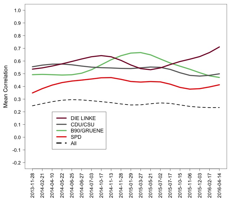
Collapsed over time we see the members of the left party agree most with each other and the members of the social democratic party agree the least with each other. The largest changes in agreement appear in the green and left party: from late 2014 to mid 2015, members of the green party seem to agree less with each other than usual, while members of the left party seem to agree more with each other than usual.

Zoom in on small Group of Members of Parliament

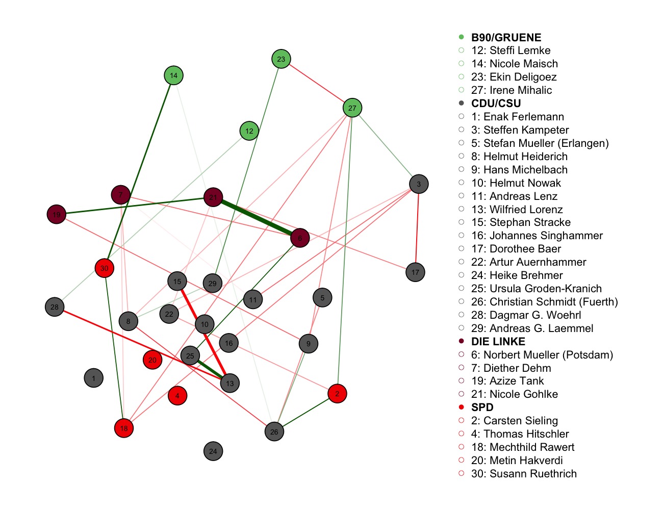
While the analyses so far gave a comprehensive overview of the voting behavior amongst members of parliament, the graph is too large to see which node in the graph corresponds to which politician. In the following graph we zoom in on a random subset of 30 politicians and match the nodes to their names:

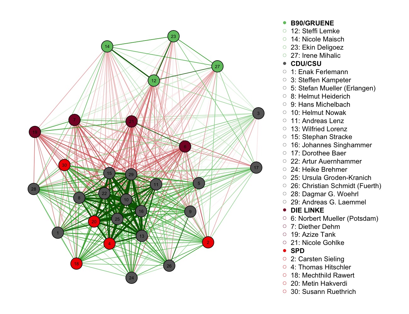
Note that correlations are bivariate measures and therefore the correlations in this smaller graph are the same as the ones in the larger graph above. We see the same overall structure as above, but now with names assigned to nodes. Again the members of the green party cluster together, but for instance Nicole Maisch votes more often together with Steffi Lempke than with the other displayed colleagues. We also see that for instance Steffen Kampeter and Christian Schmidt are both members of the convervative party, however are placed at quite distant locations in the graph (and indeed the correlation between their voting behavior is almost zero: -0.04).

Analogous to above, we now look into how voting agreement between the politicians in our subset changes over time by computing a time-varying graph as before:

We see that voting agreement changes substantially: for instance members of the opposition parties seem to agree less and less with the grand coalition until mid-2015 and then agree again more and more until the end of the period in early 2016. Some politicians seem to change their voting pattern quite dramatically: for example the voting behavior of conserviative party member Heike Bremer strongly correlates with the voting behavior of most of her party colleagues in 2014, however in late 2015 and early 2016 the correlations are close to zero. Also, interestingly, the voting behavior of conservative Steffen Kampeter tends to vote in the opposite direction than his conservative colleagues in early 2014, but then agrees more and more with them until the last recorded votes.

‘Unique’ Agreement between Members of Parliament

So far we looked into how the voting patterns of any pair of members of parliaments correlate with each other. While this is an informative measure and gives a first overview of how politicians vote relative to each other, it is also a measure that is tricky to interpret. For instance two politicians of a party might always vote together because they always align their votes with their common mentor in the party. Or because there is pressure from the whole party to vote for a bill together. Or because they are both members of a specific think tank within the parliament, …

An interesting alternative measure is conditional correlation, which is the correlation between any two members of parliament, after controlling for all other members of parliament. In case of a conditional correlation between two members of parliament there are still many possible explanations (e.g. both might be influenced by some personoutside the parliament), however, we are sure that this correlation cannot be explained by the voting pattern by any other member of parliament. We compute this conditional correlation graph and visualize it using the same layout as in the corresponding correlation graph:

It is apparent that there are less edges and less strong edges. Note that this is what we would expect in this dataset: in a parliament there is a general level of agreement within parties and also between parties, otherwise it would be difficult to pass bills. Therefore, we would expect that a substantial part of a correlation between the voting pattern between any two politicians can be explained by the voting patterns of other politicians. The strongest conditional correlations is the one between Nicole Gohlke and Norbert Mueller of the left party. For some reason these two politicians align their votes in a way that cannot be explained by the voting pattern of other politicians within and outside their party. Note here that

Concluding comments

It came as quite a surprise to me that the large majority of votes on bills in the German parliament are not recorded and hence not available to the public (please correct me if I missed something). While this is a major reason to interpret these data with caution, on the other hand the votes on bills that are recorded are the more controversial and therefore probably more interesting ones.

The graphs in this post were the first few obvious things I wanted to look into, but of course many more analyses are possible. I put the preprocessed data (no information lost, just everyting in 3 linked files instead of hundreds) on Github alongside with the code that produces the above figures. In case you have any comments, complaints or questions, please comment below!

Written on May 18, 2016

 

转自：http://jmbh.github.io//Analyzing-voting-pattern-of-German-parliament/