在本章主要内容：

NumPy基础知识
加载iris数据集
查看iris数据集
用pandas查看iris数据集
用NumPy和matplotlib绘图
最小机器学习配方 - SVM分类
介绍交叉验证
以上汇总
机器学习概述 - 分类与回归

简介

本章我们将学习如何使用scikit-learn进行预测。机器学习强调衡量预测能力，并用scikit-learn进行准确和快速的预测。我们将检查iris数据集，该数据集由三种iris的测量结果组成：Iris Setosa，Iris Versicolor和Iris Virginica。

为了衡量预测，我们将：

保存一些数据以进行测试
仅使用训练数据构建模型
测量测试集的预测能力

解决问题的方法

类别(Classification)：
非文本，比如Iris
回归
聚类
降维

技术支持 (可以加qq群：887934385）

NumPy基础

数据科学经常处理结构化的数据表。scikit-learn库需要二维NumPy数组。在本节中，您将学习

NumPy的shape和dimension

   In [1]: import numpy as np

     In [2]: np.arange(10)

     Out[2]: array([0, 1, 2, 3, 4, 5, 6, 7, 8, 9])

     In [3]: array_1 = np.arange(10)

     In [4]: array_1.shape

     Out[4]: (10,)

     In [5]: array_1.ndim

     Out[5]: 1

     In [6]: array_1.reshape((5,2))

     Out[6]:

     array([[0, 1],

            [2, 3],

            [4, 5],

            [6, 7],

            [8, 9]])

     In [7]: array_1 = array_1.reshape((5,2))

     In [8]: array_1.ndim

     Out[8]: 2

NumPy广播(broadcasting)

  In [9]: array_1 + 1

     Out[9]:

     array([[ 1,  2],

            [ 3,  4],

            [ 5,  6],

            [ 7,  8],

            [ 9, 10]])

     In [10]: array_2 = np.arange(10)

     In [11]: array_2 * array_2

     Out[11]: array([ 0,  1,  4,  9, 16, 25, 36, 49, 64, 81])

     In [12]: array_2 = array_2 ** 2 #Note that this is equivalent to array_2 *

     In [13]: array_2

     Out[13]: array([ 0,  1,  4,  9, 16, 25, 36, 49, 64, 81])

     In [14]: array_2 = array_2.reshape((5,2))

     In [15]: array_2

     Out[15]:

     array([[ 0,  1],

            [ 4,  9],

            [16, 25],

            [36, 49],

            [64, 81]])

     In [16]: array_1 = array_1 + 1

     In [17]: array_1

     Out[17]:

     array([[ 1,  2],

            [ 3,  4],

            [ 5,  6],

            [ 7,  8],

            [ 9, 10]])

     In [18]: array_1 + array_2

     Out[18]:

     array([[ 1,  3],

            [ 7, 13],

            [21, 31],

            [43, 57],

            [73, 91]])

初始化NumPy数组和dtypes

   In [19]: np.zeros((5,2))

     Out[19]:

     array([[0., 0.],

            [0., 0.],

            [0., 0.],

            [0., 0.],

            [0., 0.]])

     In [20]: np.ones((5,2), dtype = np.int)

     Out[20]:

     array([[1, 1],

            [1, 1],

            [1, 1],

            [1, 1],

            [1, 1]])

     In [21]: np.empty((5,2), dtype = np.float)

     Out[21]:

     array([[0.00000000e+000, 0.00000000e+000],

            [6.90082649e-310, 6.90082647e-310],

            [6.90072710e-310, 6.90072711e-310],

            [6.90083466e-310, 0.00000000e+000],

            [6.90083921e-310, 1.90979621e-310]])

索引

  In [22]: array_1[0,0] #Finds value in first row and first column.

     Out[22]: 1

     In [23]: array_1[0,:] # View the first row

     Out[23]: array([1, 2])

     In [24]: array_1[:,0] # view the first column

     Out[24]: array([1, 3, 5, 7, 9])

     In [25]: array_1[2:5, :]

     Out[25]:

     array([[ 5,  6],

            [ 7,  8],

            [ 9, 10]])

     In [26]: array_1

     Out[26]:

     array([[ 1,  2],

            [ 3,  4],

            [ 5,  6],

            [ 7,  8],

            [ 9, 10]])

     In [27]: array_1[2:5,0]

     Out[27]: array([5, 7, 9])

布尔数组

     In [28]: array_1 > 5

     Out[28]:

     array([[False, False],

            [False, False],

            [False,  True],

            [ True,  True],

            [ True,  True]])

     In [29]: array_1[array_1 > 5]

     Out[29]: array([ 6,  7,  8,  9, 10])

算术运算

 In [30]: array_1.sum()

     Out[30]: 55

     In [31]: array_1.sum(axis = 1) # Find all the sums by row:

     Out[31]: array([ 3,  7, 11, 15, 19])

     In [32]: array_1.sum(axis = 0) # Find all the sums by column

     Out[32]: array([25, 30])

     In [33]: array_1.mean(axis = 0)

     Out[33]: array([5., 6.])

NaN值

  # Scikit-learn不接受np.nan

     In [34]: array_3 = np.array([np.nan, 0, 1, 2, np.nan])

     In [35]: np.isnan(array_3)

     Out[35]: array([ True, False, False, False,  True])

     In [36]: array_3[~np.isnan(array_3)]

     Out[36]: array([0., 1., 2.])

     In [37]: array_3[np.isnan(array_3)] = 0

     In [38]: array_3

     Out[38]: array([0., 0., 1., 2., 0.])

Scikit-learn只接受实数的二维NumPy数组，没有缺失的np.nan值。从经验来看，最好将np.nan改为某个值丢弃。就我个人而言，我喜欢跟踪布尔模板并保持数据的形状大致相同，因为这会导致更少的编码错误和更多的编码灵活性。

加载数据

 In [1]: import numpy as np

 In [2]: import pandas as pd

 In [3]: import matplotlib.pyplot as plt

 In [4]: from sklearn import datasets

 In [5]: iris = datasets.load_iris()

 In [6]: iris.data

 Out[6]:

 array([[5.1, 3.5, 1.4, 0.2],

        [4.9, 3. , 1.4, 0.2],

        [4.7, 3.2, 1.3, 0.2],

        [4.6, 3.1, 1.5, 0.2],

        [5. , 3.6, 1.4, 0.2],

        [5.4, 3.9, 1.7, 0.4],

        [4.6, 3.4, 1.4, 0.3],

        [5. , 3.4, 1.5, 0.2],

        [4.4, 2.9, 1.4, 0.2],

        [4.9, 3.1, 1.5, 0.1],

        [5.4, 3.7, 1.5, 0.2],

        [4.8, 3.4, 1.6, 0.2],

        [4.8, 3. , 1.4, 0.1],

        [4.3, 3. , 1.1, 0.1],

        [5.8, 4. , 1.2, 0.2],

        [5.7, 4.4, 1.5, 0.4],

        [5.4, 3.9, 1.3, 0.4],

        [5.1, 3.5, 1.4, 0.3],

        [5.7, 3.8, 1.7, 0.3],

        [5.1, 3.8, 1.5, 0.3],

        [5.4, 3.4, 1.7, 0.2],

        [5.1, 3.7, 1.5, 0.4],

        [4.6, 3.6, 1. , 0.2],

        [5.1, 3.3, 1.7, 0.5],

        [4.8, 3.4, 1.9, 0.2],

        [5. , 3. , 1.6, 0.2],

        [5. , 3.4, 1.6, 0.4],

        [5.2, 3.5, 1.5, 0.2],

        [5.2, 3.4, 1.4, 0.2],

        [4.7, 3.2, 1.6, 0.2],

        [4.8, 3.1, 1.6, 0.2],

        [5.4, 3.4, 1.5, 0.4],

        [5.2, 4.1, 1.5, 0.1],

        [5.5, 4.2, 1.4, 0.2],

        [4.9, 3.1, 1.5, 0.1],

        [5. , 3.2, 1.2, 0.2],

        [5.5, 3.5, 1.3, 0.2],

        [4.9, 3.1, 1.5, 0.1],

        [4.4, 3. , 1.3, 0.2],

        [5.1, 3.4, 1.5, 0.2],

        [5. , 3.5, 1.3, 0.3],

        [4.5, 2.3, 1.3, 0.3],

        [4.4, 3.2, 1.3, 0.2],

        [5. , 3.5, 1.6, 0.6],

        [5.1, 3.8, 1.9, 0.4],

        [4.8, 3. , 1.4, 0.3],

        [5.1, 3.8, 1.6, 0.2],

        [4.6, 3.2, 1.4, 0.2],

        [5.3, 3.7, 1.5, 0.2],

        [5. , 3.3, 1.4, 0.2],

        [7. , 3.2, 4.7, 1.4],

        [6.4, 3.2, 4.5, 1.5],

        [6.9, 3.1, 4.9, 1.5],

        [5.5, 2.3, 4. , 1.3],

        [6.5, 2.8, 4.6, 1.5],

        [5.7, 2.8, 4.5, 1.3],

        [6.3, 3.3, 4.7, 1.6],

        [4.9, 2.4, 3.3, 1. ],

        [6.6, 2.9, 4.6, 1.3],

        [5.2, 2.7, 3.9, 1.4],

        [5. , 2. , 3.5, 1. ],

        [5.9, 3. , 4.2, 1.5],

        [6. , 2.2, 4. , 1. ],

        [6.1, 2.9, 4.7, 1.4],

        [5.6, 2.9, 3.6, 1.3],

        [6.7, 3.1, 4.4, 1.4],

        [5.6, 3. , 4.5, 1.5],

        [5.8, 2.7, 4.1, 1. ],

        [6.2, 2.2, 4.5, 1.5],

        [5.6, 2.5, 3.9, 1.1],

        [5.9, 3.2, 4.8, 1.8],

        [6.1, 2.8, 4. , 1.3],

        [6.3, 2.5, 4.9, 1.5],

        [6.1, 2.8, 4.7, 1.2],

        [6.4, 2.9, 4.3, 1.3],

        [6.6, 3. , 4.4, 1.4],

        [6.8, 2.8, 4.8, 1.4],

        [6.7, 3. , 5. , 1.7],

        [6. , 2.9, 4.5, 1.5],

        [5.7, 2.6, 3.5, 1. ],

        [5.5, 2.4, 3.8, 1.1],

        [5.5, 2.4, 3.7, 1. ],

        [5.8, 2.7, 3.9, 1.2],

        [6. , 2.7, 5.1, 1.6],

        [5.4, 3. , 4.5, 1.5],

        [6. , 3.4, 4.5, 1.6],

        [6.7, 3.1, 4.7, 1.5],

        [6.3, 2.3, 4.4, 1.3],

        [5.6, 3. , 4.1, 1.3],

        [5.5, 2.5, 4. , 1.3],

        [5.5, 2.6, 4.4, 1.2],

        [6.1, 3. , 4.6, 1.4],

        [5.8, 2.6, 4. , 1.2],

        [5. , 2.3, 3.3, 1. ],

        [5.6, 2.7, 4.2, 1.3],

        [5.7, 3. , 4.2, 1.2],

        [5.7, 2.9, 4.2, 1.3],

        [6.2, 2.9, 4.3, 1.3],

        [5.1, 2.5, 3. , 1.1],

        [5.7, 2.8, 4.1, 1.3],

        [6.3, 3.3, 6. , 2.5],

        [5.8, 2.7, 5.1, 1.9],

        [7.1, 3. , 5.9, 2.1],

        [6.3, 2.9, 5.6, 1.8],

        [6.5, 3. , 5.8, 2.2],

        [7.6, 3. , 6.6, 2.1],

        [4.9, 2.5, 4.5, 1.7],

        [7.3, 2.9, 6.3, 1.8],

        [6.7, 2.5, 5.8, 1.8],

        [7.2, 3.6, 6.1, 2.5],

        [6.5, 3.2, 5.1, 2. ],

        [6.4, 2.7, 5.3, 1.9],

        [6.8, 3. , 5.5, 2.1],

        [5.7, 2.5, 5. , 2. ],

        [5.8, 2.8, 5.1, 2.4],

        [6.4, 3.2, 5.3, 2.3],

        [6.5, 3. , 5.5, 1.8],

        [7.7, 3.8, 6.7, 2.2],

        [7.7, 2.6, 6.9, 2.3],

        [6. , 2.2, 5. , 1.5],

        [6.9, 3.2, 5.7, 2.3],

        [5.6, 2.8, 4.9, 2. ],

        [7.7, 2.8, 6.7, 2. ],

        [6.3, 2.7, 4.9, 1.8],

        [6.7, 3.3, 5.7, 2.1],

        [7.2, 3.2, 6. , 1.8],

        [6.2, 2.8, 4.8, 1.8],

        [6.1, 3. , 4.9, 1.8],

        [6.4, 2.8, 5.6, 2.1],

        [7.2, 3. , 5.8, 1.6],

        [7.4, 2.8, 6.1, 1.9],

        [7.9, 3.8, 6.4, 2. ],

        [6.4, 2.8, 5.6, 2.2],

        [6.3, 2.8, 5.1, 1.5],

        [6.1, 2.6, 5.6, 1.4],

        [7.7, 3. , 6.1, 2.3],

        [6.3, 3.4, 5.6, 2.4],

        [6.4, 3.1, 5.5, 1.8],

        [6. , 3. , 4.8, 1.8],

        [6.9, 3.1, 5.4, 2.1],

        [6.7, 3.1, 5.6, 2.4],

        [6.9, 3.1, 5.1, 2.3],

        [5.8, 2.7, 5.1, 1.9],

        [6.8, 3.2, 5.9, 2.3],

        [6.7, 3.3, 5.7, 2.5],

        [6.7, 3. , 5.2, 2.3],

        [6.3, 2.5, 5. , 1.9],

        [6.5, 3. , 5.2, 2. ],

        [6.2, 3.4, 5.4, 2.3],

        [5.9, 3. , 5.1, 1.8]])

 In [7]: iris.data.shape

 Out[7]: (150, 4)

 In [8]: iris.data[0]

 Out[8]: array([5.1, 3.5, 1.4, 0.2])

 In [9]: iris.feature_names

 Out[9]:

 ['sepal length (cm)',

  'sepal width (cm)',

  'petal length (cm)',

  'petal width (cm)']

 In [10]: iris.target

 Out[10]:

 array([0, 0, 0, 0, 0, 0, 0, 0, 0, 0, 0, 0, 0, 0, 0, 0, 0, 0, 0, 0, 0, 0,

        0, 0, 0, 0, 0, 0, 0, 0, 0, 0, 0, 0, 0, 0, 0, 0, 0, 0, 0, 0, 0, 0,

        0, 0, 0, 0, 0, 0, 1, 1, 1, 1, 1, 1, 1, 1, 1, 1, 1, 1, 1, 1, 1, 1,

        1, 1, 1, 1, 1, 1, 1, 1, 1, 1, 1, 1, 1, 1, 1, 1, 1, 1, 1, 1, 1, 1,

        1, 1, 1, 1, 1, 1, 1, 1, 1, 1, 1, 1, 2, 2, 2, 2, 2, 2, 2, 2, 2, 2,

        2, 2, 2, 2, 2, 2, 2, 2, 2, 2, 2, 2, 2, 2, 2, 2, 2, 2, 2, 2, 2, 2,

        2, 2, 2, 2, 2, 2, 2, 2, 2, 2, 2, 2, 2, 2, 2, 2, 2, 2])

 In [11]: iris.target.shape

 Out[11]: (150,)

 In [12]: iris.target_names

 Out[12]: array(['setosa', 'versicolor', 'virginica'], dtype='<U10')

用pandas查看数据

 import numpy as np    #Load the numpy library for fast array computations

 import pandas as pd   #Load the pandas data-analysis library

 import matplotlib.pyplot as plt   #Load the pyplot visualization library

 %matplotlib inline

 from sklearn import datasets

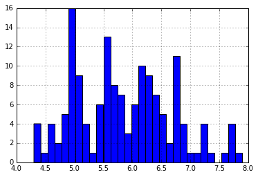
 iris = datasets.load_iris()

 iris_df = pd.DataFrame(iris.data, columns = iris.feature_names)

 iris_df['sepal length (cm)'].hist(bins=30)

```

!python

for class_number in np.unique(iris.target): plt.figure(1) iris_df['sepal length (cm)'].iloc[np.where(iris.target == class_number)[0]].hist(bins=30)

![Alt Text]({filename}/images/scikit-learn-cookbook1-pandas2.png)   

 ```

#!python

np.where(iris.target == class_number)[0]

执行结果

 array([100, 101, 102, 103, 104, 105, 106, 107, 108, 109, 110, 111, 112,

        113, 114, 115, 116, 117, 118, 119, 120, 121, 122, 123, 124, 125,

        126, 127, 128, 129, 130, 131, 132, 133, 134, 135, 136, 137, 138,

        139, 140, 141, 142, 143, 144, 145, 146, 147, 148, 149], dtype=int64)

matplotlib和NumPy作图

 import numpy as np

 import matplotlib.pyplot as plt

 %matplotlib inline

 plt.plot(np.arange(10), np.arange(10))

 plt.plot(np.arange(10), np.exp(np.arange(10)))

 # 两张图片放在一起

 plt.figure()

 plt.subplot(121)

 plt.plot(np.arange(10), np.exp(np.arange(10)))

 plt.subplot(122)

 plt.scatter(np.arange(10), np.exp(np.arange(10)))

 plt.figure()

 plt.subplot(211)

 plt.plot(np.arange(10), np.exp(np.arange(10)))

 plt.subplot(212)

 plt.scatter(np.arange(10), np.exp(np.arange(10)))

 plt.figure()

 plt.subplot(221)

 plt.plot(np.arange(10), np.exp(np.arange(10)))

 plt.subplot(222)

 plt.scatter(np.arange(10), np.exp(np.arange(10)))

 plt.subplot(223)

 plt.scatter(np.arange(10), np.exp(np.arange(10)))

 plt.subplot(224)

 plt.scatter(np.arange(10), np.exp(np.arange(10)))

 from sklearn.datasets import load_iris

 iris = load_iris()

 data = iris.data

 target = iris.target

 # Resize the figure for better viewing

 plt.figure(figsize=(12,5))

 # First subplot

 plt.subplot(121)

 # Visualize the first two columns of data:

 plt.scatter(data[:,0], data[:,1], c=target)

 # Second subplot

 plt.subplot(122)

 # Visualize the last two columns of data:

 plt.scatter(data[:,2], data[:,3], c=target)

import numpy as np

import matplotlib.pyplot as plt

%matplotlib inline

plt.plot(np.arange(10), np.arange(10))

plt.plot(np.arange(10), np.exp(np.arange(10)))

# 两张图片放在一起

plt.figure()

plt.subplot(121)

plt.plot(np.arange(10), np.exp(np.arange(10)))

plt.subplot(122)

plt.scatter(np.arange(10), np.exp(np.arange(10)))

plt.figure()

plt.subplot(211)

plt.plot(np.arange(10), np.exp(np.arange(10)))

plt.subplot(212)

plt.scatter(np.arange(10), np.exp(np.arange(10)))

plt.figure()

plt.subplot(221)

plt.plot(np.arange(10), np.exp(np.arange(10)))

plt.subplot(222)

plt.scatter(np.arange(10), np.exp(np.arange(10)))

plt.subplot(223)

plt.scatter(np.arange(10), np.exp(np.arange(10)))

plt.subplot(224)

plt.scatter(np.arange(10), np.exp(np.arange(10)))

from sklearn.datasets import load_iris

iris = load_iris()

data = iris.data

target = iris.target

# Resize the figure for better viewing

plt.figure(figsize=(12,5))

# First subplot

plt.subplot(121)

# Visualize the first two columns of data:

plt.scatter(data[:,0], data[:,1], c=target)

# Second subplot

plt.subplot(122)

# Visualize the last two columns of data:

plt.scatter(data[:,2], data[:,3], c=target)

执行结果参见

最小机器学习快速入门 - 向量机分类

为了做出预测，我们将： * 说明要解决的问题 * 选择一个模型来解决问题 * 训练模型 * 作出预测 * 衡量模型的表现如何

scikit-learn_cookbook1: 高性能机器学习-NumPy的更多相关文章

[机器学习]numpy broadcast shape 机制
最近在做机器学习的时候,对未知对webshell检测,发现代码提示:ValueError: operands could not be broadcast together with shapes ( ...
机器学习- Numpy基础吐血整理
Numpy是专门为数据科学或者数据处理相关的需求设计的一个高效的组件.听起来是不是挺绕口的,其实简单来说就2个方面,一是Numpy是专门处理数据的,二是Numpy在处理数据方面很牛逼(肯定比Pytho ...
机器学习 Numpy库入门
2017-06-28 13:56:25 Numpy 提供了一个强大的N维数组对象ndarray,提供了线性代数,傅里叶变换和随机数生成等的基本功能,可以说Numpy是Scipy,Pandas等科学计算 ...
第四十篇入门机器学习——Numpy.array的基本操作——向量及矩阵的运算
No.1. Numpy.array相较于Python原生List的性能优势 No.2. 将向量或矩阵中的每个元素 + 1 No.2. 将向量或矩阵中的所有元素 - 1 No.3. 将向量或矩阵中的所有 ...
第三十七篇入门机器学习——Numpy基础
No.1. 查看numpy版本 No.2. 为了方便使用numpy,在导入时顺便起个别名 No.3. numpy.array的基本操作:创建.查询.修改 No.4. 用dtype查看当前元素的数据类型 ...
第四十三篇入门机器学习——Numpy的基本操作——Fancy Indexing
No.1. 通过索引快速访问向量中的多个元素 No.2. 用索引对应的元素快速生成一个矩阵 No.3. 通过索引从矩阵中快速获取多个元素 No.4. 获取矩阵中感兴趣的行或感兴趣的列,重新组成矩阵 N ...
第四十二篇入门机器学习——Numpy的基本操作——索引相关
No.1. 使用np.argmin和np.argmax来获取向量元素中最小值和最大值的索引 No.2. 使用np.random.shuffle将向量中的元素顺序打乱,操作后,原向量发生改变:使用np. ...
第四十一篇入门机器学习——Numpy的基本操作——聚合操作
No.1. 对向量元素求和使用np.sum,也可以使用类似big_array.sum()的方式 No.2. 对向量元素求最小值使用np.min,求最大值使用np.max,也可以使用类似big_arra ...
第三十九篇入门机器学习——Numpy.array的基础操作——合并与分割向量和矩阵
No.1. 初始化状态 No.2. 合并多个向量为一个向量 No.3. 合并多个矩阵为一个矩阵 No.4. 借助vstack和hstack实现矩阵与向量的快速合并.或多个矩阵快速合并 No.5. 分割 ...

随机推荐

API 接口开发规范
整体规范建议采用RESTful 方式来实施. 协议 API与用户的通信协议,总是使用HTTPs协议,确保交互数据的传输安全. 域名应该尽量将API部署在专用域名之下.https://api.exam ...
在VMware下进行的Windows2008操作系统虚拟机的安装
一.VMware虚拟机的安装首先你需要拥有一款软件VMware,这是一款虚拟机安装软件.Vmware比起Vbox收费较贵,占用资源大,但是拥有大量的资源以及拥有克隆技术,适合新手学习使用,较为专业. ...
Data Deduplication Workflow Part 1
Data deduplication provides a new approach to store data and eliminate duplicate data in chunk level ...
My Eclipse 配置
设置编码格式点击Windows → preference → WorkSpace 设置编码格式点击Windows → preference → General →Appearence → Colo ...
[考试反思]0910csp-s模拟测试42：追求
显而易见的暴力骗分. T1想到了bitset但是发现MLE后弃了,部分分都没拿. T2想到正解贪心打暴力过不了大样例弃了. T3牛逼题暴力. 考场没什么大失误,还可以. 不要轻易放弃每一个思路,可能再 ...
简单搭建DNS服务器——bind
1安装bind yum install -y bind bind-utils bind-chroot 2 修改配置文件 # grep '^[^#]' /etc/named.conf options { ...
ASCALL码对照表
ASCALL码对照表目前计算机中用得最广泛的字符集及其编码,是由美国国家标准局(ANSI)制定的ASCII码(American Standard Code for Information Inter ...
C语言程序设计100例之（6）：数字反转
例6 数字反转题目描述给定一个整数,请将该数各个位上数字反转得到一个新数.新数也应满足整数的常见形式,即除非给定的原数为零,否则反转后得到的新数的最高位数字不应为零(参见样例2). 输入格式 ...
vue登录功能和将商品添加至购物车实现
2.1: 学子商城--用户登录用户登录商城用户操作行为,操作用户输入用户名和密码点击登录按钮,一种情况登录成功一种情况登录失败 "用户名或密码有误请检查" 2.2:如何实现 ...
007.Kubernetes二进制部署Flannel
一部署flannel 1.1 安装flannel kubernetes 要求集群内各节点(包括 master 节点)能通过 Pod 网段互联互通.flannel 使用 vxlan 技术为各节点创建一 ...

scikit-learn_cookbook1: 高性能机器学习-NumPy

简介