课程一(Neural Networks and Deep Learning)，第二周（Basics of Neural Network programming）—— 4、Logistic Regression with a Neural Network mindset

Logistic Regression with a Neural Network mindset

Welcome to the first (required) programming exercise of the deep learning specialization. In this notebook you will build your first image recognition algorithm. You will build a cat classifier that recognizes cats with 70% accuracy!

As you keep learning new techniques you will increase it to 80+ % accuracy on cat vs. non-cat datasets. By completing this assignment you will:

- Work with logistic regression in a way that builds intuition relevant to neural networks.

- Learn how to minimize the cost function.

- Understand how derivatives of the cost are used to update parameters.

Take your time to complete this assignment and make sure you get the expected outputs when working through the different exercises. In some code blocks, you will find a "#GRADED FUNCTION: functionName" comment. Please do not modify these comments. After you are done, submit your work and check your results. You need to score 70% to pass. Good luck :) !

中文翻译-------->

神经网络的逻辑回归

欢迎来首 (必填) 编程练习的深度学习专业化。在本笔记本中, 您将构建第一个图像识别算法。你将建立一个猫分类器, 识别猫与70% 的准确性!

随着你不断学习新的技术, 你将增加到 80 +% 的准确性 cat vs. non-cat 数据集。通过完成此任务, 您将:

 

-使用逻辑回归的方法。

-了解如何将成本函数降到最低。

-了解如何使用成本的导数来更新参数。

 

用你的时间完成这个任务, 并确保你得到预期的产出时, 通过不同的练习。在某些代码块中, 您将找到一个"#GRADED FUNCTION: functionName" 注释。请不要修改这些注释。完成后, 提交您的工作, 并检查您的结果。你需要得分70% 才能过关。祝你好运:)!

---------------------------------------------------------------------------------------------------------------------------------------------------

Logistic Regression with a Neural Network mindset

Welcome to your first (required) programming assignment! You will build a logistic regression classifier to recognize cats. This assignment will step you through how to do this with a Neural Network mindset, and so will also hone your intuitions about deep learning.

Instructions:

• Do not use loops (for/while) in your code, unless the instructions explicitly ask you to do so.

You will learn to:

• Build the general architecture of a learning algorithm, including:
  • Initializing parameters
  • Calculating the cost function and its gradient
  • Using an optimization algorithm (gradient descent)
• Gather all three functions above into a main model function, in the right order.

 中文翻译-------->

神经网络的逻辑回归

欢迎您的第一个 (必填) 编程任务!你将建立一个逻辑回归分类器来识别猫。这项任务将会让你通过神经网络思维来完成这项工作, 也会磨练你对深度学习的直觉。

说明:

不要在代码中使用循环, 除非指令明确要求您这样做。

您将学习:

1、构建学习算法的一般体系结构, 包括:

(1)初始化参数

(2)成本函数及其梯度的计算

(3)使用优化算法 (渐变下降)

2、按正确的顺序将上述所有三函数集中到一个主模型函数中。

-------------------------------------------------------------------------------------------------------------------------------------

1 - Packages

First, let's run the cell below to import all the packages that you will need during this assignment.

• numpy is the fundamental package for scientific computing with Python.
• h5py is a common package to interact with a dataset that is stored on an H5 file.
• matplotlib is a famous library to plot graphs in Python.
• PIL and scipy are used here to test your model with your own picture at the end.

code------------->

import numpy as np
import matplotlib.pyplot as plt
import h5py
import scipy
from PIL import Image
from scipy import ndimage
from lr_utils import load_dataset

%matplotlib inline

-----------------------------------------------------------------------------------------------------------------------------------------------

2 - Overview of the Problem set

Problem Statement: You are given a dataset ("data.h5") containing:

- a training set of m_train images labeled as cat (y=1) or non-cat (y=0)
- a test set of m_test images labeled as cat or non-cat
- each image is of shape (num_px, num_px, 3) where 3 is for the 3 channels (RGB). Thus, each image is square (height = num_px) and (width = num_px).

You will build a simple image-recognition algorithm that can correctly classify pictures as cat or non-cat.

Let's get more familiar with the dataset. Load the data by running the following code.

# Loading the data (cat/non-cat)
train_set_x_orig, train_set_y, test_set_x_orig, test_set_y, classes = load_dataset()

We added "_orig" at the end of image datasets (train and test) because we are going to preprocess them. After preprocessing, we will end up with train_set_x and test_set_x (the labels train_set_y and test_set_y don't need any preprocessing).

Each line of your train_set_x_orig and test_set_x_orig is an array representing an image. You can visualize an example by running the following code. Feel free also to change the index value and re-run to see other images.

中文翻译------>

我们在图像数据集 (训练和测试) 的末尾添加了 "_orig", 因为我们要对它们进行预处理。经过预处理后, 我们将得到train_set_x 和 test_set_x (标签 train_set_y 和 test_set_y 不需要任何预处理)。

train_set_x_orig 和 test_set_x_orig 的每一列都是一个表示图像的数组。您可以通过运行以下代码来可视化一个示例。也可以随意更改索引值并重新运行以查看其他图像。

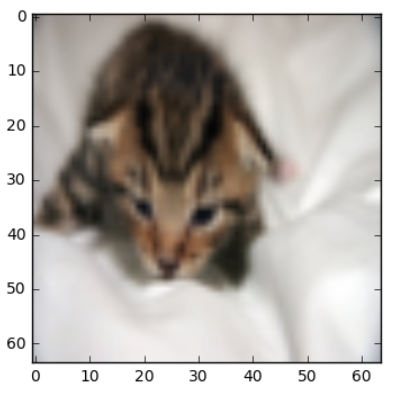
# Example of a picture
index = 25
plt.imshow(train_set_x_orig[index])
print ("y = " + str(train_set_y[:, index]) + ", it's a '" + classes[np.squeeze(train_set_y[:, index])].decode("utf-8") +  "' picture.")

result：

y = [1], it's a 'cat' picture.

-------------------------------------------------------------------------------------------------------------------------------------------------------------

Many software bugs in deep learning come from having matrix/vector dimensions that don't fit. If you can keep your matrix/vector dimensions straight you will go a long way toward eliminating many bugs.

Exercise: Find the values for:

- m_train (number of training examples)
- m_test (number of test examples)
- num_px (= height = width of a training image)

Remember that train_set_x_orig is a numpy-array of shape (m_train, num_px, num_px, 3). For instance, you can access m_train by writing train_set_x_orig.shape[0].

### START CODE HERE ### (≈ 3 lines of code)
m_train = train_set_x_orig.shape[0]
m_test =test_set_x_orig.shape[0]
num_px =train_set_x_orig.shape[1]  #train_set_x_orig= (m_train, num_px, num_px, 3).
### END CODE HERE ###

print ("Number of training examples: m_train = " + str(m_train))
print ("Number of testing examples: m_test = " + str(m_test))
print ("Height/Width of each image: num_px = " + str(num_px))
print ("Each image is of size: (" + str(num_px) + ", " + str(num_px) + ", 3)")
print ("train_set_x shape: " + str(train_set_x_orig.shape))
print ("train_set_y shape: " + str(train_set_y.shape))
print ("test_set_x shape: " + str(test_set_x_orig.shape))
print ("test_set_y shape: " + str(test_set_y.shape))

result:

Number of training examples: m_train = 209
Number of testing examples: m_test = 50
Height/Width of each image: num_px = 64
Each image is of size: (64, 64, 3)
train_set_x shape: (209, 64, 64, 3)
train_set_y shape: (1, 209)
test_set_x shape: (50, 64, 64, 3)
test_set_y shape: (1, 50)

Expected Output for m_train, m_test and num_px:

m_train	209
m_test	50
num_px	64

-------------------------------------------------------------------------------------------------------------------------------------------------------------------------------------------------------

For convenience, you should now reshape images of shape (num_px, num_px, 3) in a numpy-array of shape (num_px ∗∗ num_px ∗∗ 3, 1). After this, our training (and test) dataset is a numpy-array where each column represents a flattened image. There should be m_train (respectively m_test) columns.

Exercise: Reshape the training and test data sets so that images of size (num_px, num_px, 3) are flattened into single vectors of shape (num_px ∗∗ num_px ∗∗ 3, 1).

A trick when you want to flatten a matrix X of shape (a,b,c,d) to a matrix X_flatten of shape (b∗∗c∗∗d, a) is to use:

X_flatten = X.reshape(X.shape[0], -1).T      # X.T is the transpose of X

# Reshape the training and test examples

### START CODE HERE ### (≈ 2 lines of code)
train_set_x_flatten = train_set_x_orig.reshape(train_set_x_orig.shape[0],-1).T
test_set_x_flatten = test_set_x_orig.reshape(test_set_x_orig.shape[0],-1).T
### END CODE HERE ###

print ("train_set_x_flatten shape: " + str(train_set_x_flatten.shape))
print ("train_set_y shape: " + str(train_set_y.shape))
print ("test_set_x_flatten shape: " + str(test_set_x_flatten.shape))
print ("test_set_y shape: " + str(test_set_y.shape))
print ("sanity check after reshaping: " + str(train_set_x_flatten[0:5,0])) #整形后的完整性检查

result:

train_set_x_flatten shape: (12288, 209)
train_set_y shape: (1, 209)
test_set_x_flatten shape: (12288, 50)
test_set_y shape: (1, 50)
sanity check after reshaping: [17 31 56 22 33]

Expected Output:

train_set_x_flatten shape	(12288, 209)
train_set_y shape	(1, 209)
test_set_x_flatten shape	(12288, 50)
test_set_y shape	(1, 50)
sanity check after reshaping	[17 31 56 22 33]

---------------------------------------------------------------------------------------------------------------------------------------

To represent color images, the red, green and blue channels (RGB) must be specified for each pixel, and so the pixel value is actually a vector of three numbers ranging from 0 to 255.

One common preprocessing step in machine learning is to center and standardize your dataset, meaning that you substract the mean of the whole numpy array from each example, and then divide each example by the standard deviation of the whole numpy array. But for picture datasets, it is simpler and more convenient and works almost as well to just divide every row of the dataset by 255 (the maximum value of a pixel channel).

Let's standardize our dataset.

中文翻译------->

要表示彩色图像, 必须为每个像素指定红色、绿色和蓝色通道 (RGB), 因此像素值实际上是三数字的向量, 这些数字从0到255不等。

机器学习中一个常见的预处理步骤是中心化和标准化数据集, 这意味着您减每个示例中的整个 numpy 数组的平均值, 然后除以numpy 数组的标准差。但是对于图片数据集,可以将数据集的每一行除以 255 (像素通道的最大值)，这样更简单、更方便。

让我们标准化数据集。

What you need to remember:

Common steps for pre-processing a new dataset are:

• Figure out the dimensions and shapes of the problem (m_train, m_test, num_px, ...)
• Reshape the datasets such that each example is now a vector of size (num_px * num_px * 3, 1)
• "Standardize" the data

中文翻译------->

您需要记住的内容:

　　用于预处理新数据集的常用步骤有:

　　找出问题的尺寸和形状 (m_train, m_test, num_px,...)

　　重塑数据集, 使每个示例都是一个列向量 (num_px * num_px * 3, 1)

　　"标准化" 数据

-------------------------------------------------------------------------------------------------------------

3 - General Architecture of the learning algorithm

It's time to design a simple algorithm to distinguish cat images from non-cat images.

You will build a Logistic Regression, using a Neural Network mindset. The following Figure explains why Logistic Regression is actually a very simple Neural Network!

Mathematical expression of the algorithm:

For one example x(i)x(i):

The cost is then computed by summing over all training examples:

Key steps: In this exercise, you will carry out the following steps:

- Initialize the parameters of the model
- Learn the parameters for the model by minimizing the cost
- Use the learned parameters to make predictions (on the test set)
- Analyse the results and conclude

------------------------------------------------------------------------------------------------------------

4 - Building the parts of our algorithm

The main steps for building a Neural Network are:

1. Define the model structure (such as number of input features)
2. Initialize the model's parameters
3. Loop:
   • Calculate current loss (forward propagation)
   • Calculate current gradient (backward propagation)
   • Update parameters (gradient descent)

You often build 1-3 separately and integrate them into one function we call model().

4.1 - Helper functions(辅助函数)

Exercise: Using your code from "Python Basics", implement sigmoid(). As you've seen in the figure above, you need to compute 

to make predictions. Use np.exp().

# GRADED FUNCTION: sigmoid

def sigmoid(z):
    """
    Compute the sigmoid of z

    Arguments:
    z -- A scalar or numpy array of any size.

    Return:
    s -- sigmoid(z)
    """

    ### START CODE HERE ### (≈ 1 line of code)
    s = 1/(1+np.exp(-z))
    ### END CODE HERE ###

    return s

print ("sigmoid([0, 2]) = " + str(sigmoid(np.array([0,2]))))

result:

sigmoid([0, 2]) = [ 0.5         0.88079708]

Expected Output:

sigmoid([0, 2])

[ 0.5 0.88079708]

-----------------------------------------------------------------------------------------------------------------------------------------------------

4.2 - Initializing parameters

Exercise: Implement parameter initialization in the cell below. You have to initialize w as a vector of zeros. If you don't know what numpy function to use, look up np.zeros() in the Numpy library's documentation.

# GRADED FUNCTION: initialize_with_zeros

def initialize_with_zeros(dim):
    """
    This function creates a vector of zeros of shape (dim, 1) for w and initializes b to 0.

    Argument:
    dim -- size of the w vector we want (or number of parameters in this case)

    Returns:
    w -- initialized vector of shape (dim, 1)
    b -- initialized scalar (corresponds to the bias)
    """

    ### START CODE HERE ### (≈ 1 line of code)
    w = np.zeros((dim,1))
    b = 0
    ### END CODE HERE ###

    assert(w.shape == (dim, 1))
    assert(isinstance(b, float) or isinstance(b, int))

    return w, b

dim = 2
w, b = initialize_with_zeros(dim)
print ("w = " + str(w))
print ("b = " + str(b))

result:

w = [[ 0.]
 [ 0.]]
b = 0

Expected Output:

w	[[ 0.] [ 0.]]
b	0

For image inputs, w will be of shape (num_px ×× num_px ×× 3, 1).

----------------------------------------------------------------------------------------------------------------------------------------

4.3 - Forward and Backward propagation

Now that your parameters are initialized, you can do the "forward" and "backward" propagation steps for learning the parameters.

Exercise: Implement a function propagate()（传播函数） that computes the cost function and its gradient.

Hints(提示):

Forward Propagation:

• You get X
• You compute 
• You calculate the cost function: 

Here are the two formulas you will be using:

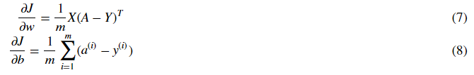
# GRADED FUNCTION: propagate

def propagate(w, b, X, Y):
    """
    Implement the cost function and its gradient for the propagation explained above

    Arguments:
    w -- weights, a numpy array of size (num_px * num_px * 3, 1)
    b -- bias, a scalar
    X -- data of size (num_px * num_px * 3, number of examples)
    Y -- true "label" vector (containing 0 if non-cat, 1 if cat) of size (1, number of examples)

    Return:
    cost -- negative log-likelihood cost for logistic regression
    dw -- gradient of the loss with respect to w, thus same shape as w
    db -- gradient of the loss with respect to b, thus same shape as b

    Tips:
    - Write your code step by step for the propagation. np.log(), np.dot()
    """

    m = X.shape[1]

    # FORWARD PROPAGATION (FROM X TO COST
    ### START CODE HERE ### (≈ 2 lines of code)
    A = sigmoid(np.add(np.dot(w.T, X), b))                                  # compute activation
    cost = -(np.dot(Y, np.log(A).T) + np.dot(1 - Y, np.log(1 - A).T)) / m                             # compute cost
    ### END CODE HERE ###

    # BACKWARD PROPAGATION (TO FIND GRAD)
    ### START CODE HERE ### (≈ 2 lines of code)
    dw = np.dot(X, (A - Y).T) / m
    db = np.sum(A - Y) / m
    ### END CODE HERE ###

    assert(dw.shape == w.shape)
    assert(db.dtype == float)
    cost = np.squeeze(cost)    #从数组的形状中删除单维条目，即把shape中为1的维度去掉
    assert(cost.shape == ())   #判断剩下的是否为空

    grads = {"dw": dw,
             "db": db}

    return grads, cost

w, b, X, Y = np.array([[1.],[2.]]), 2., np.array([[1.,2.,-1.],[3.,4.,-3.2]]), np.array([[1,0,1]])
grads, cost = propagate(w, b, X, Y)
print ("dw = " + str(grads["dw"]))
print ("db = " + str(grads["db"]))
print ("cost = " + str(cost))

result:

dw = [[ 0.99845601]
 [ 2.39507239]]
db = 0.00145557813678
cost = 5.801545319394553

Expected Output:

dw	[[ 0.99845601] [ 2.39507239]]
db	0.00145557813678
cost	5.801545319394553

 ---------------------------------------------------------------------------------------------------------------------------------------------

d) Optimization

• You have initialized your parameters.
• You are also able to compute a cost function and its gradient.
• Now, you want to update the parameters using gradient descent.

Exercise: Write down the optimization function. The goal is to learn w and bb by minimizing the cost function J. For a parameter θθ, the update rule is θ=θ−α dθθ=θ−α dθ, where αα is the learning rate.

# GRADED FUNCTION: optimize

def optimize(w, b, X, Y, num_iterations, learning_rate, print_cost = False):
    """
    This function optimizes w and b by running a gradient descent algorithm

    Arguments:
    w -- weights, a numpy array of size (num_px * num_px * 3, 1)
    b -- bias, a scalar
    X -- data of shape (num_px * num_px * 3, number of examples)
    Y -- true "label" vector (containing 0 if non-cat, 1 if cat), of shape (1, number of examples)
    num_iterations -- number of iterations of the optimization loop
    learning_rate -- learning rate of the gradient descent update rule
    print_cost -- True to print the loss every 100 steps

    Returns:
    params -- dictionary containing the weights w and bias b
    grads -- dictionary containing the gradients of the weights and bias with respect to the cost function
    costs -- list of all the costs computed during the optimization, this will be used to plot the learning curve.

    Tips:
    You basically need to write down two steps and iterate through them:
        1) Calculate the cost and the gradient for the current parameters. Use propagate().
        2) Update the parameters using gradient descent rule for w and b.
    """

    costs = []

    for i in range(num_iterations):

        # Cost and gradient calculation (≈ 1-4 lines of code)
        ### START CODE HERE ###
        grads, cost = propagate(w, b, X, Y)
        ### END CODE HERE ###

        # Retrieve derivatives from grads
        dw = grads["dw"]
        db = grads["db"]

        # update rule (≈ 2 lines of code)
        ### START CODE HERE ###
        w = w- learning_rate*dw
        b = b- learning_rate*db
        ### END CODE HERE ###

        # Record the costs
        if i % 100 == 0:
            costs.append(cost)

        # Print the cost every 100 training examples
        if print_cost and i % 100 == 0:
            print ("Cost after iteration %i: %f" %(i, cost))

    params = {"w": w,
              "b": b}

    grads = {"dw": dw,
             "db": db}

    return params, grads, costs

params, grads, costs = optimize(w, b, X, Y, num_iterations= 100, learning_rate = 0.009, print_cost = False)

print ("w = " + str(params["w"]))
print ("b = " + str(params["b"]))
print ("dw = " + str(grads["dw"]))
print ("db = " + str(grads["db"]))

result:

w = [[ 0.19033591]
 [ 0.12259159]]
b = 1.92535983008
dw = [[ 0.67752042]
 [ 1.41625495]]
db = 0.219194504541

Expected Output:

w	[[ 0.19033591] [ 0.12259159]]
b	1.92535983008
dw	[[ 0.67752042] [ 1.41625495]]
db	0.219194504541

Exercise: The previous function will output the learned w and b. We are able to use w and b to predict the labels for a dataset X. Implement the predict()function. There is two steps to computing predictions:

1. Calculate 

2. Convert the entries of a into 0 (if activation <= 0.5) or 1 (if activation > 0.5), stores the predictions in a vector Y_prediction. If you wish, you can use an if/else statement in a for loop (though there is also a way to vectorize this).

# GRADED FUNCTION: predict

def predict(w, b, X):
    '''
    Predict whether the label is 0 or 1 using learned logistic regression parameters (w, b)

    Arguments:
    w -- weights, a numpy array of size (num_px * num_px * 3, 1)
    b -- bias, a scalar
    X -- data of size (num_px * num_px * 3, number of examples)

    Returns:
    Y_prediction -- a numpy array (vector) containing all predictions (0/1) for the examples in X
    '''

    m = X.shape[1]    #样本数
    Y_prediction = np.zeros((1,m))
    w = w.reshape(X.shape[0], 1)

    # Compute vector "A" predicting the probabilities of a cat being present in the picture
    ### START CODE HERE ### (≈ 1 line of code)
    A =  sigmoid(np.add(np.dot(w.T, X), b))  #(1,m)
    ### END CODE HERE ###

    for i in range(A.shape[1]):

        # Convert probabilities A[0,i] to actual predictions p[0,i]
        ### START CODE HERE ### (≈ 4 lines of code)
        if A[0,i]<=0.5:
             Y_prediction[0,i]= 0
        else:
             Y_prediction[0,i]= 1
        ### END CODE HERE ###

    assert(Y_prediction.shape == (1, m))

    return Y_prediction

w = np.array([[0.1124579],[0.23106775]])
b = -0.3
X = np.array([[1.,-1.1,-3.2],[1.2,2.,0.1]])
print ("predictions = " + str(predict(w, b, X)))

result:

predictions = [[ 1.  1.  0.]]

Expected Output:

predictions

[[ 1. 1. 0.]]

What to remember: You've implemented several functions that:

• Initialize (w,b)
• Optimize the loss iteratively to learn parameters (w,b):
  • computing the cost and its gradient
  • updating the parameters using gradient descent
• Use the learned (w,b) to predict the labels for a given set of examples

中文翻译------>

要记住的内容: 您已经实现了以下几个功能:

初始化 (w, b)

迭代地优化损失函数，学习参数 (w, b):

　　计算成本函数及其梯度

　　使用梯度下降算法来更新参数

使用所学 (w, b) 来预测给定标签的数据集

----------------------------------------------------------------------------------------------------------------------------

5 - Merge all functions into a model

You will now see how the overall model is structured by putting together all the building blocks (functions implemented in the previous parts) together, in the right order.

Exercise: Implement the model function. Use the following notation:

- Y_prediction for your predictions on the test set
- Y_prediction_train for your predictions on the train set
- w, costs, grads for the outputs of optimize()

# GRADED FUNCTION: model

def model(X_train, Y_train, X_test, Y_test, num_iterations = 2000, learning_rate = 0.5, print_cost = False):
    """
    Builds the logistic regression model by calling the function you've implemented previously

    Arguments:
    X_train -- training set represented by a numpy array of shape (num_px * num_px * 3, m_train)
    Y_train -- training labels represented by a numpy array (vector) of shape (1, m_train)
    X_test -- test set represented by a numpy array of shape (num_px * num_px * 3, m_test)
    Y_test -- test labels represented by a numpy array (vector) of shape (1, m_test)
    num_iterations -- hyperparameter representing the number of iterations to optimize the parameters
    learning_rate -- hyperparameter representing the learning rate used in the update rule of optimize()
    print_cost -- Set to true to print the cost every 100 iterations

    Returns:
    d -- dictionary containing information about the model.
    """

    ### START CODE HERE ###

    # initialize parameters with zeros (≈ 1 line of code)
    w, b = initialize_with_zeros(X_train.shape[0])

    # Gradient descent (≈ 1 line of code)
    parameters, grads, costs = optimize(w, b, X_train, Y_train, num_iterations, learning_rate, print_cost)

    # Retrieve parameters w and b from dictionary "parameters"
    w = parameters["w"]
    b = parameters["b"]

    # Predict test/train set examples (≈ 2 lines of code)
    Y_prediction_test = predict(w, b, X_test)
    Y_prediction_train = predict(w, b, X_train)
    ### END CODE HERE ###

    # Print train/test Errors
    print("train accuracy: {} %".format(100 - np.mean(np.abs(Y_prediction_train - Y_train)) * 100))
    print("test accuracy: {} %".format(100 - np.mean(np.abs(Y_prediction_test - Y_test)) * 100))

    d = {"costs": costs,
         "Y_prediction_test": Y_prediction_test,
         "Y_prediction_train" : Y_prediction_train,
         "w" : w,
         "b" : b,
         "learning_rate" : learning_rate,
         "num_iterations": num_iterations}

    return d

Run the following cell to train your model.

d = model(train_set_x, train_set_y, test_set_x, test_set_y, num_iterations =2000, learning_rate = 0.005, print_cost = True)

Cost after iteration 0: 0.693147
Cost after iteration 100: 0.584508
Cost after iteration 200: 0.466949
Cost after iteration 300: 0.376007
Cost after iteration 400: 0.331463
Cost after iteration 500: 0.303273
Cost after iteration 600: 0.279880
Cost after iteration 700: 0.260042
Cost after iteration 800: 0.242941
Cost after iteration 900: 0.228004
Cost after iteration 1000: 0.214820
Cost after iteration 1100: 0.203078
Cost after iteration 1200: 0.192544
Cost after iteration 1300: 0.183033
Cost after iteration 1400: 0.174399
Cost after iteration 1500: 0.166521
Cost after iteration 1600: 0.159305
Cost after iteration 1700: 0.152667
Cost after iteration 1800: 0.146542
Cost after iteration 1900: 0.140872
train accuracy: 99.04306220095694 %
test accuracy: 70.0 %

Expected Output:

Cost after iteration 0	0.693147
⋮⋮	⋮⋮
Train Accuracy	99.04306220095694 %
Test Accuracy	70.0 %

Comment: Training accuracy is close to 100%. This is a good sanity check: your model is working and has high enough capacity to fit the training data. Test error is 68%. It is actually not bad for this simple model, given the small dataset we used and that logistic regression is a linear classifier. But no worries, you'll build an even better classifier next week!

Also, you see that the model is clearly overfitting the training data. Later in this specialization you will learn how to reduce overfitting, for example by using regularization. Using the code below (and changing the index variable) you can look at predictions on pictures of the test set.

中文翻译------->

备注: 训练集预测的准确度接近100%。这是一个很好的健全检查: 您的模型是有效的, 有足够高的能力， 适应训练数据。测试集预测的错误率为68%。对个简单的模型，这个结果实际上是不坏的。因为我们使用的小数据集和逻辑回归是一个线性分类器。但不用担心, 下周你会建立一个更好的分类器!

此外, 您还可以看到模型显然过拟合了训练数据。在本专业后期, 您将学习如何减少过拟合, 例如使用正则化。使用下面的代码 (并更改索引变量), 您可以查看测试集的预测结果以及对应的图片。

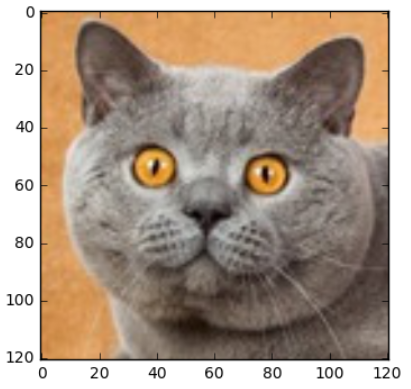
# Example of a picture that was wrongly classified.
index =1
plt.imshow(test_set_x[:,index].reshape((num_px, num_px, 3)))
print ("y = " + str(test_set_y[0,index]) + ", you predicted that it is a \"" + classes[d["Y_prediction_test"][0,index]].decode("utf-8") +  "\" picture.")

result:

y = 1, you predicted that it is a "cat" picture.

Let's also plot the cost function and the gradients.

# Plot learning curve (with costs)
costs = np.squeeze(d['costs'])
plt.plot(costs)
plt.ylabel('cost')
plt.xlabel('iterations (per hundreds)')
plt.title("Learning rate =" + str(d["learning_rate"]))
plt.show()

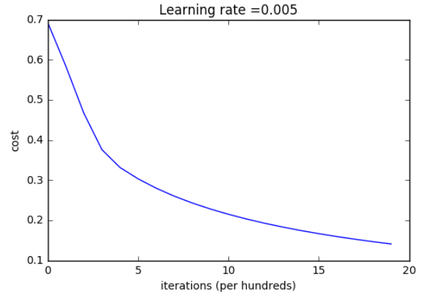
Interpretation: You can see the cost decreasing. It shows that the parameters are being learned. However, you see that you could train the model even more on the training set. Try to increase the number of iterations in the cell above and rerun the cells. You might see that the training set accuracy goes up, but the test set accuracy goes down. This is called overfitting.

-----------------------------------------------------------------------------------------------------------------------------------

6 - Further analysis (optional/ungraded exercise)

Congratulations on building your first image classification model. Let's analyze it further, and examine possible choices for the learning rate α.

Choice of learning rate

Reminder: In order for Gradient Descent to work you must choose the learning rate wisely. The learning rate αα determines how rapidly we update the parameters. If the learning rate is too large we may "overshoot" the optimal value. Similarly, if it is too small we will need too many iterations to converge to the best values. That's why it is crucial to use a well-tuned learning rate.

Let's compare the learning curve of our model with several choices of learning rates. Run the cell below. This should take about 1 minute. Feel free also to try different values than the three we have initialized the learning_rates variable to contain, and see what happens.

learning_rates = [0.01, 0.001, 0.0001]
models = {}
for i in learning_rates:
    print ("learning rate is: " + str(i))
    models[str(i)] = model(train_set_x, train_set_y, test_set_x, test_set_y, num_iterations = 1500, learning_rate = i, print_cost = False)
    print ('\n' + "-------------------------------------------------------" + '\n')

for i in learning_rates:
    plt.plot(np.squeeze(models[str(i)]["costs"]), label= str(models[str(i)]["learning_rate"]))

plt.ylabel('cost')
plt.xlabel('iterations')

legend = plt.legend(loc='upper center', shadow= True)
frame = legend.get_frame()
frame.set_facecolor('0.90')
plt.show()

result:

learning rate is: 0.01
train accuracy: 99.52153110047847 %
test accuracy: 68.0 %

-------------------------------------------------------

learning rate is: 0.001
train accuracy: 88.99521531100478 %
test accuracy: 64.0 %

-------------------------------------------------------

learning rate is: 0.0001
train accuracy: 68.42105263157895 %
test accuracy: 36.0 %

-------------------------------------------------------

Interpretation:

• Different learning rates give different costs and thus different predictions results.
• If the learning rate is too large (0.01), the cost may oscillate up and down. It may even diverge (though in this example, using 0.01 still eventually ends up at a good value for the cost).
• A lower cost doesn't mean a better model. You have to check if there is possibly overfitting. It happens when the training accuracy is a lot higher than the test accuracy.
• In deep learning, we usually recommend that you:
  • Choose the learning rate that better minimizes the cost function.
  • If your model overfits, use other techniques to reduce overfitting. (We'll talk about this in later videos.)

中文翻译------->

解释:

不同的学习速率用于代价函数，因而得到不同的预测结果。

如果学习速率太大 (0.01), 成本可能会上下摆动。它甚至可能会发散 (虽然在这个例子中, 使用0.01 最终仍然到了一个很好的代价函数的值)。

较低的代价函数值并不意味着更好的模型。你必须检查是否过拟合。当训练精度比测试精度高很多时, 就会发生这种情况。

在深入学习中, 我们通常建议您:

选择更好地降低代价函数的学习速率。

如果您的模型过拟合了, 可以使用其他技术减少过拟合。(我们将在以后的视频中讨论此事)

----------------------------------------------------------------------------------------------------------------------------------

7 - Test with your own image (optional/ungraded exercise)

Congratulations on finishing this assignment. You can use your own image and see the output of your model. To do that:

1. Click on "File" in the upper bar of this notebook, then click "Open" to go on your Coursera Hub.
2. Add your image to this Jupyter Notebook's directory, in the "images" folder
3. Change your image's name in the following code
4. Run the code and check if the algorithm is right (1 = cat, 0 = non-cat)!

中文翻译--------------->

1. 单击本笔记本栏中的 "文件", 然后单击 "打开" 进入您的 Coursera Hub。

2. 将您的图像添加到此 Jupyter 笔记本的目录中, 在 "图像" 文件夹中

3. 在下面的代码中更改图像的名称

4. 运行代码并检查算法是否正确 (1 = cat, 0 = non-cat)!

 

code1----------------->

## START CODE HERE ## (PUT YOUR IMAGE NAME)
my_image = "my_cat.jpg"   # change this to the name of your image file
## END CODE HERE ##

# We preprocess the image to fit your algorithm.
fname = "images/" + my_image
image = np.array(ndimage.imread(fname, flatten=False))
my_image = scipy.misc.imresize(image, size=(num_px,num_px)).reshape((1, num_px*num_px*3)).T   #待解释
my_predicted_image = predict(d["w"], d["b"], my_image)

plt.imshow(image)
print("y = " + str(np.squeeze(my_predicted_image)) + ", your algorithm predicts a \"" + classes[int(np.squeeze(my_predicted_image)),].decode("utf-8") +  "\" picture.")

result:

y = 1.0, your algorithm predicts a "cat" picture.

code2--------------------->

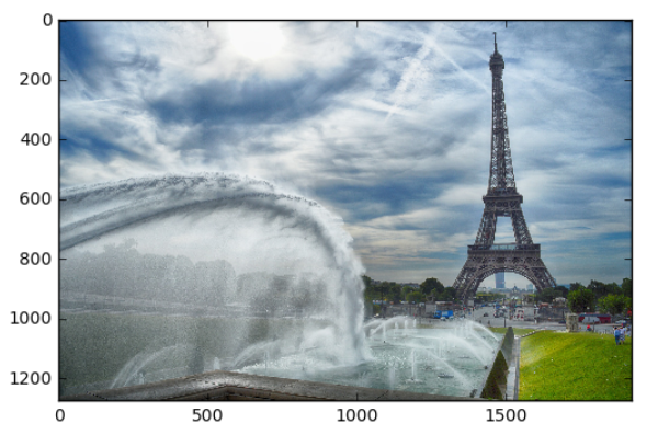
## START CODE HERE ## (PUT YOUR IMAGE NAME)
my_image = "my_image.jpg"   # change this to the name of your image file
## END CODE HERE ##

# We preprocess the image to fit your algorithm.
fname = "images/" + my_image
image = np.array(ndimage.imread(fname, flatten=False))
my_image = scipy.misc.imresize(image, size=(num_px,num_px)).reshape((1, num_px*num_px*3)).T   #待解释
my_predicted_image = predict(d["w"], d["b"], my_image)

plt.imshow(image)
print("y = " + str(np.squeeze(my_predicted_image)) + ", your algorithm predicts a \"" + classes[int(np.squeeze(my_predicted_image)),].decode("utf-8") +  "\" picture.")

result:

y = 0.0, your algorithm predicts a "non-cat" picture.

What to remember from this assignment:

• Preprocessing the dataset is important.
• You implemented each function separately: initialize(), propagate(), optimize(). Then you built a model().
• Tuning the learning rate (which is an example of a "hyperparameter") can make a big difference to the algorithm. You will see more examples of this later in this course!

--------------------------------------------------------------------------------------------------------------------------------------------

Finally, if you'd like, we invite you to try different things on this Notebook. Make sure you submit before trying anything. Once you submit, things you can play with include:

- Play with the learning rate and the number of iterations
- Try different initialization methods and compare the results
- Test other preprocessings (center the data, or divide each row by its standard deviation)

中文翻译-------->

最后, 如果你想, 我们邀请你尝试不同的东西在这个笔记本上。在尝试任何事情之前, 请务必提交。一旦你提交, 你可以玩的东西包括:

-尝试不同的学习速率和迭代次数

-尝试不同的初始化方法并比较结果

-测试其他 预处理方法 (中心化数据, 或除以每行的标准差)

 

Bibliography(书目):
- http://www.wildml.com/2015/09/implementing-a-neural-network-from-scratch/
- https://stats.stackexchange.com/questions/211436/why-do-we-normalize-images-by-subtracting-the-datasets-image-mean-and-not-the-c