chapter2 线性回归实现

1 导入包

import numpy as np

2 初始化模型参数

### 初始化模型参数
def initialize_params(dims):
    w = np.zeros((dims, 1))
    b = 0
    return w, b

3 损失函数计算

### 包括线性回归公式、均方损失和参数偏导三部分
def linear_loss(X, y, w, b):
    num_train = X.shape[0]
    y_hat = np.dot(X, w) + b
    # 计算预测输出与实际标签之间的均方损失
    loss = np.sum((y_hat-y)**2)/num_train
    # 基于均方损失对权重参数的一阶偏导数
    dw = 2*np.dot(X.T, (y_hat-y)) /num_train
    # 基于均方损失对偏差项的一阶偏导数
    db = 2*np.sum((y_hat-y)) /num_train
    return y_hat, loss, dw, db

4 定义线性回归模型训练过程

### 定义线性回归模型训练过程
def linear_train(X, y, learning_rate=0.01, epochs=10000):
    loss_his = []
    # 初始化模型参数
    w, b = initialize_params(X.shape[1])
    for i in range(1, epochs):
        # 计算当前迭代的预测值、损失和梯度
        y_hat, loss, dw, db = linear_loss(X, y, w, b)
        # 基于梯度下降的参数更新
        w += -learning_rate * dw
        b += -learning_rate * db
        # 记录当前迭代的损失
        loss_his.append(loss)
        # 每1000次迭代打印当前损失信息
        if i % 10000 == 0:
            print('epoch %d loss %f' % (i, loss))
        params = {
            'w': w,
            'b': b
        }
        grads = {
            'dw': dw,
            'db': db
        }
    return loss_his, params, grads

5 导入数据集并划分数据集

from sklearn.datasets import load_diabetes
from sklearn.utils import shuffle
diabetes = load_diabetes()
data, target = diabetes.data, diabetes.target
X, y = shuffle(data, target, random_state=13)
# 按照8/2划分训练集和测试集
offset = int(X.shape[0] * 0.8)
X_train, y_train = X[:offset], y[:offset].reshape((-1,1))
X_test, y_test = X[offset:], y[offset:].reshape((-1,1))
# 打印训练集和测试集维度
print("X_train's shape: ", X_train.shape)
print("X_test's shape: ", X_test.shape)
print("y_train's shape: ", y_train.shape)
print("y_test's shape: ", y_test.shape)

结果：

X_train's shape:  (353, 10)
X_test's shape:  (89, 10)
y_train's shape:  (353, 1)
y_test's shape:  (89, 1)

6 线性回归模型训练

# 线性回归模型训练
loss_his, params, grads = linear_train(X_train, y_train, 0.01, 200000)
# 打印训练后得到模型参数
print(params)

结果：

epoch 10000 loss 3219.178670
epoch 20000 loss 2944.940452
epoch 30000 loss 2848.052938
epoch 40000 loss 2806.628090
epoch 50000 loss 2788.051589
epoch 60000 loss 2779.411239
epoch 70000 loss 2775.230777
epoch 80000 loss 2773.107175
epoch 90000 loss 2771.957481
epoch 100000 loss 2771.281723
epoch 110000 loss 2770.843500
epoch 120000 loss 2770.528226
epoch 130000 loss 2770.278899
epoch 140000 loss 2770.066388
epoch 150000 loss 2769.875394
epoch 160000 loss 2769.697658
epoch 170000 loss 2769.528602
epoch 180000 loss 2769.365613
epoch 190000 loss 2769.207165
{'w': array([[   9.84972769],
       [-240.38803204],
       [ 491.45462983],
       [ 298.20492926],
       [ -87.77291402],
       [ -98.36201742],
       [-186.17374049],
       [ 177.38726503],
       [ 424.17405761],
       [  52.48952427]]), 'b': 150.8136201371859}

7 定义线性回归预测函数

### 定义线性回归预测函数
def predict(X, params):
    w = params['w']
    b = params['b']
    y_pred = np.dot(X, w) + b
    return y_pred
y_pred = predict(X_test, params)

8 定义R2系数函数

### 定义R2系数函数
def r2_score(y_test, y_pred):
    # 测试标签均值
    y_avg = np.mean(y_test)
    # 总离差平方和
    ss_tot = np.sum((y_test - y_avg)**2)
    # 残差平方和
    ss_res = np.sum((y_test - y_pred)**2)
    # R2计算
    r2 = 1 - (ss_res/ss_tot)
    return r2

print(r2_score(y_test, y_pred))

结果：

0.5349331079250876

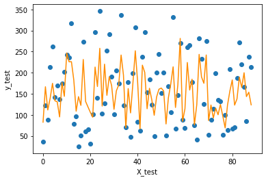
9 可视化

import matplotlib.pyplot as plt
f = X_test.dot(params['w']) + params['b']

plt.scatter(range(X_test.shape[0]), y_test)
plt.plot(f, color = 'darkorange')
plt.xlabel('X_test')
plt.ylabel('y_test')
plt.show();

结果：

　　

plt.plot(loss_his, color = 'blue')
plt.xlabel('epochs')
plt.ylabel('loss')
plt.show()

结果：

　　

10 手写交叉验证

from sklearn.utils import shuffle
X, y = shuffle(data, target, random_state=13)
X = X.astype(np.float32)
data = np.concatenate((X, y.reshape((-1,1))), axis=1)
data.shape

结果：

(442, 11)

from random import shuffle
def k_fold_cross_validation(items, k, randomize=True):
    if randomize:
        items = list(items)
        shuffle(items)
    slices = [items[i::k] for i in range(k)]
    for i in range(k):
        validation = slices[i]
        training = [item
                    for s in slices if s is not validation
                    for item in s]
        training = np.array(training)
        validation = np.array(validation)
        yield training, validation
for training, validation in k_fold_cross_validation(data, 5):
    X_train = training[:, :10]
    y_train = training[:, -1].reshape((-1,1))
    X_valid = validation[:, :10]
    y_valid = validation[:, -1].reshape((-1,1))
    loss5 = []
    #print(X_train.shape, y_train.shape, X_valid.shape, y_valid.shape)
    loss, params, grads = linear_train(X_train, y_train, 0.001, 100000)
    loss5.append(loss)
    score = np.mean(loss5)
    print('five kold cross validation score is', score)
    y_pred = predict(X_valid, params)
    valid_score = np.sum(((y_pred-y_valid)**2))/len(X_valid)
    print('valid score is', valid_score)

结果：

epoch 10000 loss 5092.953795
epoch 20000 loss 4625.210998
epoch 30000 loss 4280.106579
epoch 40000 loss 4021.857859
epoch 50000 loss 3825.526402
epoch 60000 loss 3673.689068
epoch 70000 loss 3554.135457
epoch 80000 loss 3458.274820
epoch 90000 loss 3380.033392
five kold cross validation score is 4095.209897465298
valid score is 3936.2234811935696
epoch 10000 loss 5583.270165
epoch 20000 loss 5048.748757
epoch 30000 loss 4655.620298
epoch 40000 loss 4362.817211
epoch 50000 loss 4141.575958
epoch 60000 loss 3971.714077
epoch 70000 loss 3839.037331
epoch 80000 loss 3733.533571
epoch 90000 loss 3648.114252
five kold cross validation score is 4447.019807745928
valid score is 2501.3520150018944
epoch 10000 loss 5200.950784
epoch 20000 loss 4730.397070
epoch 30000 loss 4382.133800
epoch 40000 loss 4120.944891
epoch 50000 loss 3922.113137
epoch 60000 loss 3768.255158
epoch 70000 loss 3647.113946
epoch 80000 loss 3550.018924
epoch 90000 loss 3470.811373
five kold cross validation score is 4191.91819552402
valid score is 3599.5500530218555
epoch 10000 loss 5392.825769
epoch 20000 loss 4859.145634
epoch 30000 loss 4465.914858
epoch 40000 loss 4172.706513
epoch 50000 loss 3951.112149
epoch 60000 loss 3781.128244
epoch 70000 loss 3648.633504
epoch 80000 loss 3543.627226
epoch 90000 loss 3458.998687
five kold cross validation score is 4256.231602795183
valid score is 3306.6604398106706
epoch 10000 loss 4991.290783
epoch 20000 loss 4547.454621
epoch 30000 loss 4219.702158
epoch 40000 loss 3974.018034
epoch 50000 loss 3786.721727
epoch 60000 loss 3641.292905
epoch 70000 loss 3526.175261
epoch 80000 loss 3433.256913
epoch 90000 loss 3356.818661
five kold cross validation score is 4043.189167421097
valid score is 4220.025355059865

11 导入数据集

from sklearn.datasets import load_diabetes
from sklearn.utils import shuffle
from sklearn.model_selection import train_test_split

diabetes = load_diabetes()
data = diabetes.data
target = diabetes.target
X, y = shuffle(data, target, random_state=13)
X = X.astype(np.float32)
y = y.reshape((-1, 1))
X_train, X_test, y_train, y_test = train_test_split(X, y, test_size=0.2, random_state=42)
print(X_train.shape, y_train.shape, X_test.shape, y_test.shape)

结果：

(353, 10) (353, 1) (89, 10) (89, 1)

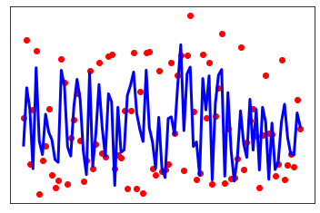
11 sklearn实现，并可视化

import matplotlib.pyplot as plt
import numpy as np
from sklearn import linear_model
from sklearn.metrics import mean_squared_error, r2_score
regr = linear_model.LinearRegression()
regr.fit(X_train, y_train)
y_pred = regr.predict(X_test)
# The coefficients
print('Coefficients: \n', regr.coef_)
# The mean squared error
print("Mean squared error: %.2f"
      % mean_squared_error(y_test, y_pred))
# Explained variance score: 1 is perfect prediction
print('Variance score: %.2f' % r2_score(y_test, y_pred))
print(r2_score(y_test, y_pred))

# Plot outputs
plt.scatter(range(X_test.shape[0]), y_test, color='red')
plt.plot(range(X_test.shape[0]), y_pred, color='blue', linewidth=3)
plt.xticks(())
plt.yticks(())
plt.show();

结果：

Coefficients:
 [[ -23.51037 -216.31213  472.36694  372.07175 -863.6967   583.2741
   105.79268  194.76984  754.073     38.2222 ]]
Mean squared error: 3028.50
Variance score: 0.53
0.5298198993375712

　　

12 交叉验证

from sklearn.model_selection import KFold
from sklearn.linear_model import LinearRegression
### 交叉验证
def cross_validate(model, x, y, folds=5, repeats=5):
    ypred = np.zeros((len(y),repeats))
    score = np.zeros(repeats)
    for r in range(repeats):
        i=0
        print('Cross Validating - Run', str(r + 1), 'out of', str(repeats))
        x,y = shuffle(x, y, random_state=r) #shuffle data before each repeat
        kf = KFold(n_splits=folds,random_state=i+1000,shuffle=True) #random split, different each time
        for train_ind, test_ind in kf.split(x):
            print('Fold', i+1, 'out of', folds)
            xtrain,ytrain = x[train_ind,:],y[train_ind]
            xtest,ytest = x[test_ind,:],y[test_ind]
            model.fit(xtrain, ytrain)
            #print(xtrain.shape, ytrain.shape, xtest.shape, ytest.shape)
            ypred[test_ind]=model.predict(xtest)
            i+=1
        score[r] = r2_score(ypred[:,r],y)
    print('\nOverall R2:',str(score))
    print('Mean:',str(np.mean(score)))
    print('Deviation:',str(np.std(score)))
    pass

cross_validate(regr, X, y, folds=5, repeats=5)

结果：

Cross Validating - Run 1 out of 5
Fold 1 out of 5
Fold 2 out of 5
Fold 3 out of 5
Fold 4 out of 5
Fold 5 out of 5
Cross Validating - Run 2 out of 5
Fold 1 out of 5
Fold 2 out of 5
Fold 3 out of 5
Fold 4 out of 5
Fold 5 out of 5
Cross Validating - Run 3 out of 5
Fold 1 out of 5
Fold 2 out of 5
Fold 3 out of 5
Fold 4 out of 5
Fold 5 out of 5
Cross Validating - Run 4 out of 5
Fold 1 out of 5
Fold 2 out of 5
Fold 3 out of 5
Fold 4 out of 5
Fold 5 out of 5
Cross Validating - Run 5 out of 5
Fold 1 out of 5
Fold 2 out of 5
Fold 3 out of 5
Fold 4 out of 5
Fold 5 out of 5

Overall R2: [0.03209418 0.04484132 0.02542677 0.01093105 0.02690136]
Mean: 0.028038935700747846
Deviation: 0.010950454328955226