《MATLAB Deep Learning:With Machine Learning,Neural Networks and Artificial Intelligence》选记
一、Training of a Single-Layer Neural Network
1 Delta Rule
Consider a single-layer neural network, as shown in Figure 2-11. In the figure, d i is the correct output of the output node i.

Long story short, the delta rule adjusts the weight as the following algorithm:
“If an input node contributes to the error of the output node, the weight between the two nodes is adjusted in proportion to the input value, x j and the output error, e i .”
This rule can be expressed in equation as:
where
x j = The output from the input node j, ( j =1 2 3 , , )
e i = The error of the output node i
w ij = The weight between the output node i and input
node j
α = Learning rate (0 <α<=1 )
note: The learning rate, α, determines how much the weight is changed per time.
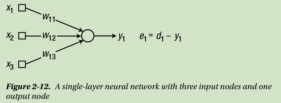
Note that the first number of the subscript (1) indicates the node number to which the input enters. For example, the weight between the input node 2 and output node 1 is denoted as w 12 . This notation enables an easier matrix operation; the weights associated with the node i are allocated at the i -th row of the weight matrix.Applying the delta rule of Equation 2.2 to the example neural network yields the renewal of the weights as:

Let’s summarize the training process using the delta rule for the single-layer neural network.
1. Initialize the weights at adequate values.
2. Take the “input” from the training data of { input, correct output } and enter it to the neural network.Calculate the error of the output, yi , from the correct output, di , to the input.

3. Calculate the weight updates according to the following delta rule:

4. Adjust the weights as:

5. Perform Steps 2-4 for all training data.
6. Repeat Steps 2-5 until the error reaches an acceptable tolerance level.
note:
Just for reference, the number of training iterations, in each of which all
training data goes through Steps 2-5 once, is called an epoch. For instance,
epoch = 10 means that the neural network goes through 10 repeated training
processes with the same dataset.

2 Generalized Delta Rule
The delta rule of the previous section is rather obsolete. Later studies
have uncovered that there exists a more generalized form of the delta rule. For
an arbitrary activation function, the delta rule is expressed as the following
equation.

It is the same as the delta rule of the previous section, except that ei is replaced with δi . In this equation, δi is defined as:
where
e i = The error of the output node i
v i = The weighted sum of the output node i
φ′ = The derivative of the activation function φ of the output node i

Plugging this equation into Equation 2.3 results in the same formula as the
delta rule in Equation 2.2. This fact indicates that the delta rule in Equation 2.2 is
only valid for linear activation functions.
Now, we can derive the delta rule with the sigmoid function, which is widely
used as an activation function. The sigmoid function is defined as shown in
Figure 2-14.

We need the derivative of this function, which is given as:

Substituting this derivative into Equation 2.4 yields δ i as:

Again, plugging this equation into Equation 2.3 gives the delta rule for the sigmoid function as:

Although the weight update formula is rather complicated, it maintains the identical fundamental concept where the weight is determined in proportion to the output node error, ei and the input node value, xj
二、SGD, Batch, and Mini Batch
The schemes that are used to calculate the weight update, ∆wij , are introduced in this section. Three typical schemes are available for supervised learning of the neural network.
1 Stochastic Gradient Descent
The Stochastic Gradient Descent (SGD) calculates the error for each training data and adjusts the weights immediately. If we have 100 training data points,the SGD adjusts the weights 100 times.
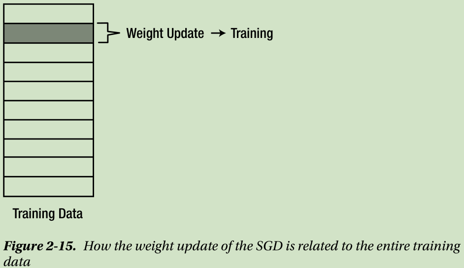
As the SGD adjusts the weight for each data point, the performance of the neural network is crooked while the undergoing the training process. The name “stochastic” implies the random behavior of the training process. The SGD calculates the weight updates as:

This equation implies that all the delta rules of the previous sections are based on the SGD approach.
2 Batch
In the batch method, each weight update is calculated for all errors of the training data, and the average of the weight updates is used for adjusting the weights. This method uses all of the training data and updates only once.
The batch method calculates the weight update as:

where ∆wij(k) is the weight update for the k -th training data and N is the total number of the training data.
Because of the averaged weight update calculation, the batch method consumes a significant amount of time for training。
The batch method requires more time to train the neural network to yield a similar level of accuracy of that of the SGD method. In other words, the batch method learns slowly.
3 Mini Batch
The mini batch method is a blend of the SGD and batch methods. It selects a part of the training dataset and uses them for training in the batch method. Therefore,it calculates the weight updates of the selected data and trains the neural network with the averaged weight update. For example, if 20 arbitrary data points are selected out of 100 training data points, the batch method is applied to the 20 data points. In this case, a total of five weight adjustments are performed to complete the training process for all the data points (5 = 100/20).

The mini batch method, when it selects an appropriate number of data points, obtains the benefits from both methods: speed from the SGD and stability from the batch. For this reason, it is often utilized in Deep Learning,which manipulates a significant amount of data.
note:As previously addressed, the SGD trains every data point immediately and does not require addition or averages of the weight updates. Therefore, the code for the SGD is simpler than that of the batch.
三、Training of Multi-Layer Neural Network
The previously introduced delta rule is ineffective for training of the multi-layer neural network. This is because the error, the essential element for applying the delta rule for training, is not defined in the hidden layers. The error of the output node is defined as the difference between the correct output and the output of the neural network. However, the training data does not provide correct outputs for the hidden layer nodes, and hence the error cannot be calculated using the same approach for the output nodes. Then, what? Isn’t the real problem how to define the error at the hidden nodes? You got it. You just formulated the back-propagation algorithm, the representative learning rule of the multi-layer neural network.
The significance of the back-propagation algorithm was that it provided a systematic method to determine the error of the hidden nodes. Once the hidden layer errors are determined, the delta rule is applied to adjust the weights.
四、Cost Function (It is also called the loss function and objective function) and Learning Rule
The cost function is a rather mathematical concept that is associated with the optimization theory.
the measure of the neural network’s error is the cost function. The greater the error of the neural network, the higher the value of the cost function is. There are two primary types of cost functions for the neural network’s supervised learning.
where y i is the output from the output node, d i is the correct output from the training data, and M is the number of output nodes.
First, consider the sum of squared error shown in Equation 3.9. This cost function is the square of the difference between the neural network’s output, y,and the correct output, d. If the output and correct output are the same, the error becomes zero. In contrast, a greater difference between the two values leads to a larger error. This is illustrated in Figure 3-9.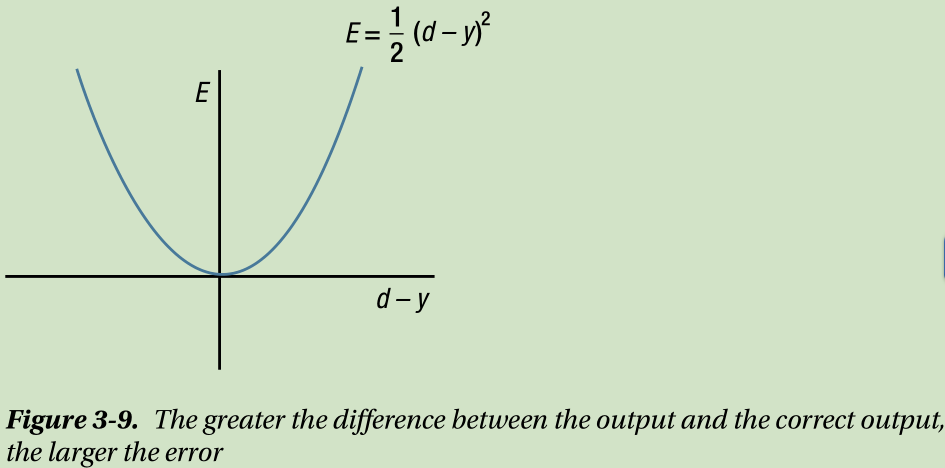
Most early studies of the neural network employed this cost function to derive learning rules. Not only was the delta rule of the previous chapter derived from this function, but the back-propagation algorithm was as well. Regression problems still use this cost function.
Now, consider the cost function of Equation 3.10. The following formula, which is inside the curly braces, is called the cross entropy function.

It may be difficult to intuitively capture the cross entropy function’s relationship to the error. This is because the equation is contracted for simpler expression. Equation 3.10 is the concatenation of the following two equations:

Due to the definition of a logarithm, the output, y, should be within 0 and 1. Therefore, the cross entropy cost function often teams up with sigmoid and softmax activation functions in the neural network.
Now we will see how this function is related to the error. Recall that cost functions should be proportional to the output error. What about this one? Figure 3-10 shows the cross entropy function at d = 1 .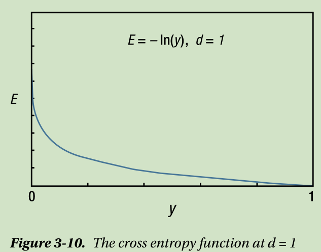
note:
If the other activation function is employed, the definition of the cross entropy function slightly changes as well.
When the output y is 1, i.e., the error (d-y ) is 0, the cost function value is 0 as well. In contrast, when the output y approaches 0, i.e., the error grows, the cost function value soars. Therefore, this cost function is proportional to the error.
Figure 3-11 shows the cost function at d = 0 . If the output y is 0, the error is 0, the cost function yields 0. When the output approaches 1, i.e., the error grows, the function value soars. Therefore, this cost function in this case is proportional to the error as well. These cases confirm that the cost function of Equation 3.10 is proportional to the output error of the neural network.
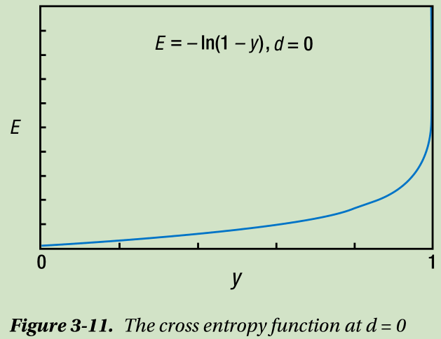
The primary difference of the cross entropy function from the quadratic function of Equation 3.9 is its geometric increase. In other words, the cross entropy function is much more sensitive to the error. For this reason, the learning rules derived from the cross entropy function are generally known to yield better performance. It is recommended that you use the cross entropy-driven learning rules except for inevitable cases such as the regression.
We had a long introduction to the cost function because the selection of the cost function affects the learning rule, i.e., the formula of the back-propagation algorithm. Specifically, the calculation of the delta at the output node changes slightly. The following steps detail the procedure in training the neural network with the sigmoid activation function at the output node using the cross entropy-driven back-propagation algorithm.
1. Initialize the neural network’s weights with adequate values.
2. Enter the input of the training data { input, correct output } to the neural network and obtain the output.Compare this output to the correct output, calculate the error, and calculate the delta, δ, of the output nodes.
3. Propagate the delta of the output node backward and calculate the delta of the subsequent hidden nodes.
4. Repeat Step 3 until it reaches the hidden layer that is next to the input layer.
5. Adjust the neural network’s weights using the following learning rule:
6. Repeat Steps 2-5 for every training data point.
7. Repeat Steps 2-6 until the network has been adequately trained.
Did you notice the difference between this process and that of the “Back-Propagation Algorithm” section? It is the delta, δ, in Step 2. It has been changed as follows:
Everything else remains the same. On the outside, the difference seems insignificant. However, it contains the huge topic of the cost function based on the optimization theory. Most of the neural network training approaches of Deep Learning employ the cross entropy-driven learning rules. This is due to
their superior learning rate and performance.
Figure 3-12 depicts what this section has explained so far. The key is the fact that the output and hidden layers employ the different formulas of the delta calculation when the learning rule is based on the cross entropy and the sigmoid function.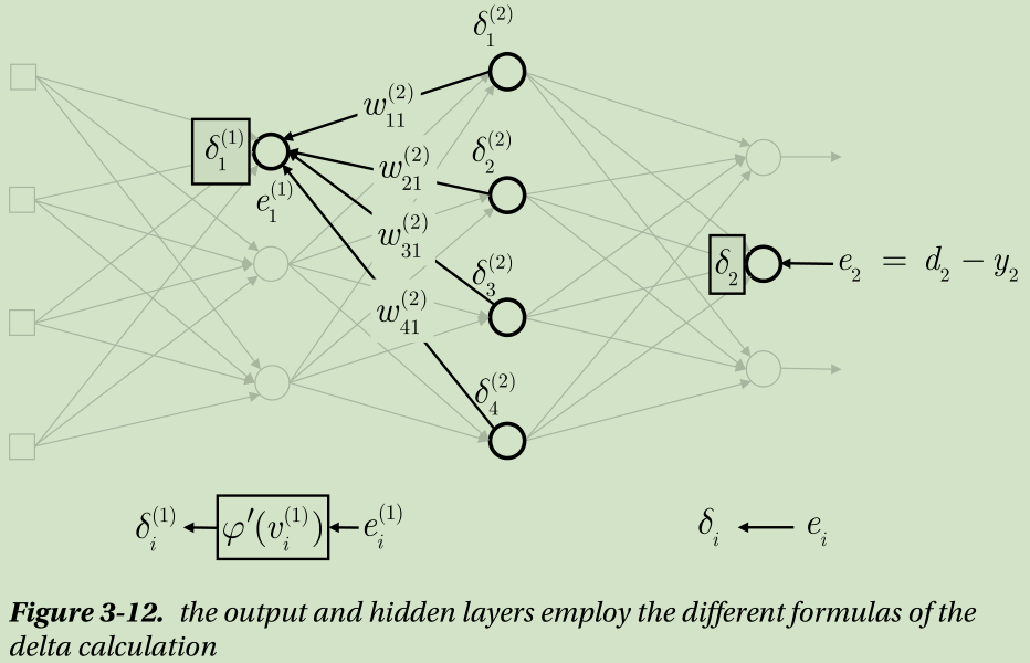
Overfitting is a challenging problem that every technique of Machine Learning faces. You also saw that one of the primary approaches used to overcome overfitting is making the model as simple as possible using regularization. In a mathematical sense, the essence of regularization is adding the sum of the weights to the cost function, as shown here. Of course, applying the following new cost function leads to a different learning rule formula.
Where λ is the coefficient that determines how much of the connection weight is reflected on the cost function.
This cost function maintains a large value when one of the output errors and the weight remain large. Therefore, solely making the output error zero will not suffice in reducing the cost function. In order to drop the value of the cost function,both the error and weight should be controlled to be as small as possible. However,if a weight becomes small enough, the associated nodes will be practically disconnected. As a result, unnecessary connections are eliminated, and the neural network becomes simpler. For this reason, overfitting of the neural network can be improved by adding the sum of weights to the cost function, thereby reducing it.
In summary, the learning rule of the neural network’s supervised learning is derived from the cost function. The performance of the learning rule and the neural network varies depending on the selection of the cost function. The cross entropy function has been attracting recent attention for the cost function. The regularization process that is used to deal with overfitting is implemented as a variation of the cost function.
Unlike the previous example code, the derivative of the sigmoid function no longer exists. This is because, for the learning rule of the cross entropy function,if the activation function of the output node is the sigmoid, the delta equals the output error.
the cross entropy-driven learning rule yields a faster learning process. This is the reason that most cost functions for Deep Learning employ the cross entropy function.
Summary
The importance of the back-propagation algorithm is that it provides a systematic method to define the error of the hidden node.
The single-layer neural network is applicable only to linearly separable problems, and most practical problems are linearly inseparable.
The multi-layer neural network is capable of modeling the linearly inseparable problems.
The development of various weight adjustment approaches is due to the pursuit of a more stable and faster learning of the network.
The cost function addresses the output error of the neural network and is proportional to the error.
The learning rule of the neural network varies depending on the cost function and activation function. Specifically, the delta calculation of the output node is changed.
The regularization, which is one of the approaches used to overcome overfitting, is also implemented as an addition of the weight term to the cost function.
五、Neural Network and Classification
1 binary classification
The learning process of the binary classification neural network is summarized in the following steps. Of course, we use the cross entropy function as the cost function and the sigmoid function as the activation function of the hidden and output nodes.
1. The binary classification neural network has one node for the output layer. The sigmoid function is used for the activation function.
2. Switch the class titles of the training data into numbers using the maximum and minimum values of the sigmoid function.
Class △ -> 1
Class ● -> 0
3. Initialize the weights of the neural network with adequate values.
4. Enter the input from the training data { input, correct output } into the neural network and obtain the output. Calculate the error between the output and correct output, and determine the delta, δ, of the output nodes.
5. Propagate the output delta backwards and calculate the delta of the subsequent hidden nodes.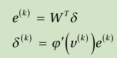
6. Repeat Step 5 until it reaches the hidden layer on the immediate right of the input layer.
7. Adjust the weights of the neural network using this learning rule:
8. Repeat Steps 4-7 for all training data points.
9. Repeat Steps 4-8 until the neural network has been trained properly.
Although it appears complicated because of its many steps, this process is basically the same as that of the back-propagation of Chapter 3. The detailed explanations are omitted.
2 multiclass classification
In general, multiclass classifiers employ the softmax function as the activation function of the output node.
The activation functions that we have discussed so far, including the sigmoid function, account only for the weighted sum of inputs. They do not consider the output from the other output nodes. However, the softmax function accounts not only for the weighted sum of the inputs, but also for the inputs to the other output nodes.
Why do we insist on using the softmax function? Consider the sigmoid function in place of the softmax function. Assume that the neural network produced the output shown in Figure 4-11 when given the input data. As the sigmoid function concerns only its own output, the output here will be generated.
adequate interpretation of the output from the multiclass classification neural network requires consideration of the relative magnitudes of all node outputs.
The softmax function maintains the sum of the output values to be one and also limits the individual outputs to be within the values of 0-1. As it accounts for the relative magnitudes of all the outputs, the softmax function is a suitable choice for the multiclass classification neural networks.
The output from the i-th output node of the softmax function is calculated as follows:
where, v i is the weighted sum of the i-th output node, and M is the number of output nodes. Following this definition, the softmax function satisfies the following condition:
Finally, the learning rule should be determined. The multiclass classification neural network usually employs the cross entropy-driven learning rules just like the binary classification network does. This is due to the high learning performance and simplicity that the cross entropy function provides.
Long story short, the learning rule of the multiclass classification neural network is identical to that of the binary classification neural network of the previous section. Although these two neural networks employ different activation functions—the sigmoid for the binary and the softmax for the multiclass—the derivation of the learning rule leads to the same result. Well, it is better for us to have less to remember.The training process of the multiclass classification neural network is summarized in these steps.
1. Construct the output nodes to have the same value as the number of classes. The softmax function is used as the activation function.
2. Switch the names of the classes into numeric vectors via the one-hot encoding method.
Class 1 -> [ 1 0 0 ]
Class 2 -> [ 0 1 0 ]
Class 3 -> [ 0 0 1 ]
3. Initialize the weights of the neural network with adequate values.
4. Enter the input from the training data { input, correct output } into the neural network and obtain the output.Calculate the error between the output and correct output and determine the delta, δ, of the output nodes.
5. Propagate the output delta backwards and calculate the delta of the subsequent hidden nodes.
6. Repeat Step 5 until it reaches the hidden layer on the immediate right of the input layer.
7. Adjust the weights of the neural network using this learning rule:

8. Repeat Steps 4-7 for all the training data points.
9. Repeat Steps 4-8 until the neural network has been trained properly.
Of course, the multiclass classification neural network is applicable for binary classification. All we have to do is construct a neural network with two
output nodes and use the softmax function as the activation function.
the practical data does not necessarily reflect the training data.This fact, as we previously discussed, is the fundamental problem of Machine Learning and needs to solve.
3 Summary
For the neural network classifier, the selection of the number of output nodes and activation function usually depends on whether it is for a binary classification (two classes) or for a multiclass classification (three or more classes).
For binary classification, the neural network is constructed with a single output node and sigmoid activation function. The correct output of the training data is converted to the maximum and minimum values of the activation function. The cost function of the learning rule employs the cross entropy function.
For a multiclass classification, the neural network includes as many output nodes as the number of classes. The softmax function is employed for the activation function of the output node. The correct output of the training data is converted into a vector using the one-hot encoding method. The cost function of the learning rule employs the cross entropy function.
《MATLAB Deep Learning:With Machine Learning,Neural Networks and Artificial Intelligence》选记的更多相关文章
- Learning How To Code Neural Networks
原文:https://medium.com/learning-new-stuff/how-to-learn-neural-networks-758b78f2736e#.ly5wpz44d This i ...
- 1506.01186-Cyclical Learning Rates for Training Neural Networks
1506.01186-Cyclical Learning Rates for Training Neural Networks 论文中提出了一种循环调整学习率来训练模型的方式. 如下图: 通过循环的线 ...
- 《Learning scikit-learn Machine Learning in Python》chapter1
前言 由于实验原因,准备入坑 python 机器学习,而 python 机器学习常用的包就是 scikit-learn ,准备先了解一下这个工具.在这里搜了有 scikit-learn 关键字的书,找 ...
- 吴恩达《深度学习》-课后测验-第一门课 (Neural Networks and Deep Learning)-Week 3 - Shallow Neural Networks(第三周测验 - 浅层神 经网络)
Week 3 Quiz - Shallow Neural Networks(第三周测验 - 浅层神经网络) \1. Which of the following are true? (Check al ...
- Paper Reading - Deep Captioning with Multimodal Recurrent Neural Networks ( m-RNN ) ( ICLR 2015 ) ★
Link of the Paper: https://arxiv.org/pdf/1412.6632.pdf Main Points: The authors propose a multimodal ...
- Machine Learning - 第6周(Advice for Applying Machine Learning、Machine Learning System Design)
In Week 6, you will be learning about systematically improving your learning algorithm. The videos f ...
- Machine Learning - XI. Machine Learning System Design机器学习系统的设计(Week 6)
http://blog.csdn.net/pipisorry/article/details/44119187 机器学习Machine Learning - Andrew NG courses学习笔记 ...
- deep learning and machine learning
http://blog.csdn.net/xiangz_csdn/article/details/54580053
- 神经网络作业: NN LEARNING Coursera Machine Learning(Andrew Ng) WEEK 5
在WEEK 5中,作业要求完成通过神经网络(NN)实现多分类的逻辑回归(MULTI-CLASS LOGISTIC REGRESSION)的监督学习(SUOERVISED LEARNING)来识别阿拉伯 ...
随机推荐
- office 激活教程
首先在我的百度云里下载:http://pan.baidu.com/share/link?shareid=2200272243&uk=1985086665激活工具安装包 如果遇到问题,可以加我Q ...
- generator详解
generator函数 yield可以返回值,也可以传入值 形式: 注意!generator不能写成arrow function的形式!!! function *函数(){ 代码1... let a ...
- Bash基本功能
bash的基本功能 作者:尹正杰 版权声明:原创作品,谢绝转载!否则将追究法律责任. 欢迎加入: 高级运维工程师之路 598432640 一.历史命令和命令补全 1.历 ...
- 机器学习课程-第8周-聚类(Clustering)—K-Mean算法
1. 聚类(Clustering) 1.1 无监督学习: 简介 在一个典型的监督学习中,我们有一个有标签的训练集,我们的目标是找到能够区分正样本和负样本的决策边界,在这里的监督学习中,我们有一系列标签 ...
- VUE2.0 饿了吗视频学习笔记(一):VUE示例data.json
https://gitee.com/1981633/vue_study.git 源码下载地址,随笔记动态更新中有的同学找不到data.json,以下是data.json内容 { "selle ...
- OpenCV入门(1)- 简介
1.图像的表示 在计算机看来,图像只是一些亮度各异的点,一副M*N的图片可以用M*N的矩阵来表示,矩阵的值表示这个位置上像素的亮度. 一般灰度图用二维矩阵来表示,彩色(多通道)图用三维矩阵表示,大部分 ...
- Linux 之【辨析UPDATE/UPGRADE】和安装/卸载软件(apt-get)
一.[辨析UPDATE/UPGRADE] UPDATE: update is used to download package information from all configured sour ...
- mysql 原理 ~ checkpoint
一 简介:今天咱们来聊聊checkpoint 二 定义: checkpoin是重做日志对数据页刷新到磁盘的操作做的检查点,通过LSN号保存记录,作用是当发生宕机等crash情况时,再次启动时会查询ch ...
- Handler实现与机制 && Blocking Queue && IdleHandler使用
http://blog.csdn.net/boyupeng/article/details/46685343 IdleHandler处理消息的源码 final Message next() { ... ...
- Struts局部异常与全局异常处理
aaarticlea/png;base64,iVBORw0KGgoAAAANSUhEUgAAAowAAAG3CAIAAACxBJNyAAAgAElEQVR4nOy9z6tk15Ymdv4B0eRU8O
