Interpolation in MATLAB

Mathematics

One-Dimensional Interpolation

There are two kinds of one-dimensional interpolation in MATLAB:

• Polynomial interpolation
• FFT-based interpolation

Polynomial Interpolation

The function interp1 performs one-dimensional interpolation, an important operation for data analysis and curve fitting. This function uses polynomial techniques, fitting the supplied data with polynomial functions between data points and evaluating the appropriate function at the desired interpolation points. Its most general form is

• yi = interp1(x,y,xi,method)
  

y is a vector containing the values of a function, and x is a vector of the same length containing the points for which the values in y are given. xi is a vector containing the points at which to interpolate. method is an optional string specifying an interpolation method:

• Nearest neighbor interpolation (method = 'nearest'). This method sets the value of an interpolated point to the value of the nearest existing data point.
• Linear interpolation (method = 'linear'). This method fits a different linear function between each pair of existing data points, and returns the value of the relevant function at the points specified by xi. This is the default method for the interp1 function.
• Cubic spline interpolation (method = 'spline'). This method fits a different cubic function between each pair of existing data points, and uses the spline function to perform cubic spline interpolation at the data points.
• Cubic interpolation (method = 'pchip' or 'cubic'). These methods are identical. They use the pchip function to perform piecewise cubic Hermite interpolation within the vectors x and y. These methods preserve monotonicity and the shape of the data.

If any element of xi is outside the interval spanned by x, the specified interpolation method is used for extrapolation. Alternatively, yi = interp1(x,Y,xi,method,extrapval) replaces extrapolated values with extrapval. NaN is often used for extrapval.

All methods work with nonuniformly spaced data.

Speed, Memory, and Smoothness Considerations

When choosing an interpolation method, keep in mind that some require more memory or longer computation time than others. However, you may need to trade off these resources to achieve the desired smoothness in the result.

• Nearest neighbor interpolation is the fastest method. However, it provides the worst results in terms of smoothness.
• Linear interpolation uses more memory than the nearest neighbor method, and requires slightly more execution time. Unlike nearest neighbor interpolation its results are continuous, but the slope changes at the vertex points.
• Cubic spline interpolation has the longest relative execution time, although it requires less memory than cubic interpolation. It produces the smoothest results of all the interpolation methods. You may obtain unexpected results, however, if your input data is non-uniform and some points are much closer together than others.
• Cubic interpolation requires more memory and execution time than either the nearest neighbor or linear methods. However, both the interpolated data and its derivative are continuous.

The relative performance of each method holds true even for interpolation of two-dimensional or multidimensional data. For a graphical comparison of interpolation methods, see the section Comparing Interpolation Methods.

FFT-Based Interpolation

The function interpft performs one-dimensional interpolation using an FFT-based method. This method calculates the Fourier transform of a vector that contains the values of a periodic function. It then calculates the inverse Fourier transform using more points. Its form is

• y = interpft(x,n)
  

x is a vector containing the values of a periodic function, sampled at equally spaced points. n is the number of equally spaced points to return.

MATLAB Function Reference

interp1

One-dimensional data interpolation (table lookup)

Syntax

• yi = interp1(x,Y,xi)
  yi = interp1(Y,xi)
  yi = interp1(x,Y,xi,method)
  yi = interp1(x,Y,xi,method,'extrap')
  yi = interp1(x,Y,xi,method,extrapval)
  

Description

yi = interp1(x,Y,xi) returns vector yi containing elements corresponding to the elements of xi and determined by interpolation within vectors x and Y. The vector x specifies the points at which the data Y is given. If Y is a matrix, then the interpolation is performed for each column of Y and yi is length(xi)-by-size(Y,2).

yi = interp1(Y,xi) assumes that x = 1:N, where N is the length of Y for vector Y, or size(Y,1) for matrix Y.

yi = interp1(x,Y,xi,method) interpolates using alternative methods:

'nearest'	Nearest neighbor interpolation
'linear'	Linear interpolation (default)
'spline'	Cubic spline interpolation
'pchip'	Piecewise cubic Hermite interpolation
'cubic'	(Same as 'pchip')
'v5cubic'	Cubic interpolation used in MATLAB 5

For the 'nearest', 'linear', and 'v5cubic' methods, interp1(x,Y,xi,method) returns NaN for any element of xi that is outside the interval spanned by x. For all other methods, interp1 performs extrapolation for out of range values.

yi = interp1(x,Y,xi,method,'extrap') uses the specified method to perform extrapolation for out of range values.

yi = interp1(x,Y,xi,method,extrapval) returns the scalar extrapval for out of range values. NaN and 0 are often used for extrapval.

The interp1 command interpolates between data points. It finds values at intermediate points, of a one-dimensional function  that underlies the data. This function is shown below, along with the relationship between vectors x, Y, xi, and yi.

Interpolation is the same operation as table lookup. Described in table lookup terms, the table is [x,Y] and interp1 looks up the elements of xi in x, and, based upon their locations, returns values yi interpolated within the elements of Y.

Note    interp1q is quicker than interp1 on non-uniformly spaced data because it does no input checking. For interp1q to work properly, x must be a monotonically increasing column vector and Y must be a column vector or matrix with length(X) rows. Type help interp1q at the command line for more information.

Examples

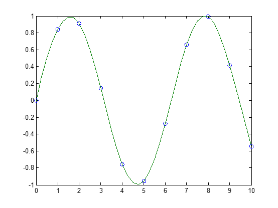
Example 1. Generate a coarse sine curve and interpolate over a finer abscissa.

• x = 0:10;
  y = sin(x);
  xi = 0:.25:10;
  yi = interp1(x,y,xi);
  plot(x,y,'o',xi,yi)

  

• with 'spline' method:

x = 0:10;

　　　y = sin(x);

xi = 0:.25:10;

        yi = interp1(x,y,xi,'spline'); 

        figure;plot(x,y,'o',xi,yi)

　　

Example 2. Here are two vectors representing the census years from 1900 to 1990 and the corresponding United States population in millions of people.

• t = 1900:10:1990;
  p = [75.995  91.972  105.711  123.203  131.669...
       150.697  179.323  203.212  226.505  249.633];
  

The expression interp1(t,p,1975) interpolates within the census data to estimate the population in 1975. The result is

• ans =
      214.8585
  

Now interpolate within the data at every year from 1900 to 2000, and plot the result.

•  x = 1900:1:2000;
   y = interp1(t,p,x,'spline');
   plot(t,p,'o',x,y)

  

Sometimes it is more convenient to think of interpolation in table lookup terms, where the data are stored in a single table. If a portion of the census data is stored in a single 5-by-2 table,

• tab =
      1950    150.697
      1960    179.323
      1970    203.212
      1980    226.505
      1990    249.633
  

then the population in 1975, obtained by table lookup within the matrix tab, is

• p = interp1(tab(:,1),tab(:,2),1975)
  p =
      214.8585
  

Algorithm

The interp1 command is a MATLAB M-file. The 'nearest' and 'linear' methods have straightforward implementations.

For the 'spline' method, interp1 calls a function spline that uses the functions ppval, mkpp, and unmkpp. These routines form a small suite of functions for working with piecewise polynomials. spline uses them to perform the cubic spline interpolation. For access to more advanced features, see the spline reference page, the M-file help for these functions, and the Spline Toolbox.

For the 'pchip' and 'cubic' methods, interp1 calls a function pchip that performs piecewise cubic interpolation within the vectors x and y. This method preserves monotonicity and the shape of the data. See the pchip reference page for more information.

See Also

interpft, interp2, interp3, interpn, pchip, spline

References

[1]  de Boor, C., A Practical Guide to Splines, Springer-Verlag, 1978.