airway之workflow

1）airway简介

在该workflow中，所用的数据集来自RNA-seq，气道平滑肌细胞(airway  smooth muscle cells )用氟美松（糖皮质激素，抗炎药）处理。例如，哮喘患者使用糖皮质激素来减少呼吸道炎症，在该实验设计中，4种细胞类型(airway smooth muscle cell lines )用1微米地塞米松处理18个小时。每一个cell lines都有对照与处理组(a treated and an untreated sample).关于实验设计的更多信息可以查看PubMed entry 24926665 ，原始数据 GEO entry GSE52778.

2）Preparing count matrices(准备制作表达矩阵)

这个矩阵必须是原始的表达量，不能是任何矫正过的表达量(RPKM等)。因为DESeq2的统计模型在处理原始表达矩阵会展示出强大实力，且会自动处理library size differences。

2.1 Aligning reads to a reference genome

for f in 'cat files'
do
    STAR --genomeDir ../STAR/ENSEMBL.homo_sapiens.release-75 --readFilesIn fastq/$f\_1.fastq fastq/$f\_2.fastq --runThreadN 12 --outFileNamePrefix aligned/$f.
done   #比对

for f in 'cat files'
do
    samtools view -bS aligned/$f.Aligned.out.sam -o aligned/$f.bam; done  #转bam文件
done

因为按照原文献跑流程，则数据量太大，耗时间，因此在airway中只用了8个样本的一些子集，来减少运行时间及内存。

library("airway")
dir <- system.file("extdata", package="airway", mustWork=TRUE)  #查看数据集所在路径
list.files(dir)
csvfile <- file.path(dir,"sample_table.csv")         #文件所在绝对路径
(sampleTable <- read.csv(csvfile,row.names=1))       #读取表格
filenames <- file.path(dir, paste0(sampleTable$Run, "_subset.bam"))
file.exists(filenames)                               #验证这8个文件在不
library("Rsamtools")
bamfiles <- BamFileList(filenames, yieldSize=2000000)  #提取2000000序列，降低时间和消耗，文件1：用于构建assay信息
seqinfo(bamfiles[1])                                   #查看信息

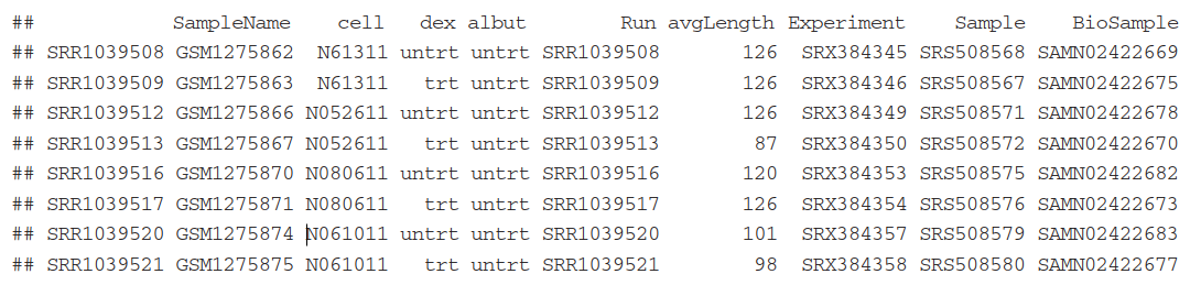
sampleTable信息：

2.2 Defining gene models( 最主要的一步是构建TxDb 对象)

Next, we need to read in the gene model that will be used for counting reads/fragments.Here,we want to make a list of exons grouped  by gene for counting read/fragments.

如果是自己的数据，首先下载gtf/gff3文件，并用GenomicFeatures 包中的makeTxDbFromGFF()函数构建TxDb object。(TxDb对象是一个包含frange-based objects, such as exons, transcripts, and genes)

library("GenomicFeatures")
gtffile <- file.path(dir,"Homo_sapiens.GRCh37.75_subset.gtf")    #airway测试自带的gtf文件，自己的数据需要下载gtf文件
(txdb <- makeTxDbFromGFF(gtffile, format="gtf", circ_seqs=character())) #读取gtf文件构建TxDb object对象
(ebg <- exonsBy(txdb, by="gene")) #构建外显子groped by gene ，文件2：rowRanges()信息

2.3 Read counting step

上述准备工作做完之后，统计表达量非常简单。 利用GenomicAlignments包中的summarizeOverlaps()函数，返回一个包含多种信息的SummarizedExperiment 对象。同时由于数据量大，对于一个包含30 million aligned reads的单个文件，summarizeOverlaps()函数至少需要30 minutes。为了节省时间可以利用BiocParallel包中的register()函数进行多核运行。

register(SerialParam()) #设置多核运行
se <- summarizeOverlaps(features=ebg, reads=bamfiles,    #创建SummarizedExperiment object with counts，上面文件1和2
                        mode="Union",            # describes what kind of read overlaps will be counted.
                        singleEnd=FALSE,        ######表示是pair-end
                        ignore.strand=TRUE,   ##是否是链特异性 strand-specific
                        fragments=TRUE )      ##specify if unpaired reads should be counted
save(se,file='count_matrix.Rdata')

2.4 SummarizedExperiment

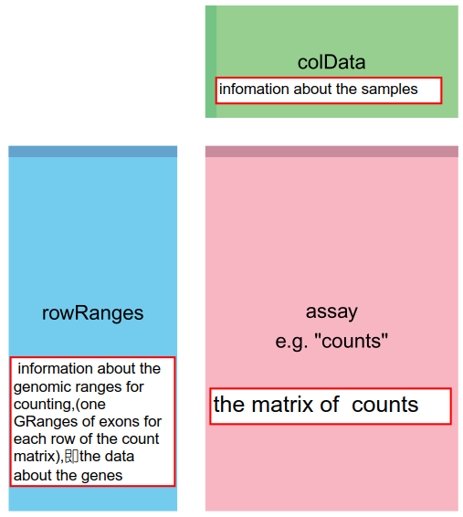
上述产生的SummarizedExperiment 对象，由3部分组成：粉色框是表达矩阵(matrix of counts,)储存在assay中，如果是多个矩阵可以储存在assays当中。浅蓝色框是rowRanges，包含genomic ranges的信息，及gtf中的gene model信息。绿色框包含样本信息(information about the samples)。

dim(se)               ## [1] 20 8
assayNames(se)        ## "counts"
head(assay(se), 3)    #查看表达矩阵
colSums(assay(se))
rowRanges(se)         #rowRanges信息
str(metadata(rowRanges(se)))  #metadata是构建基因模型的gtf文件信息
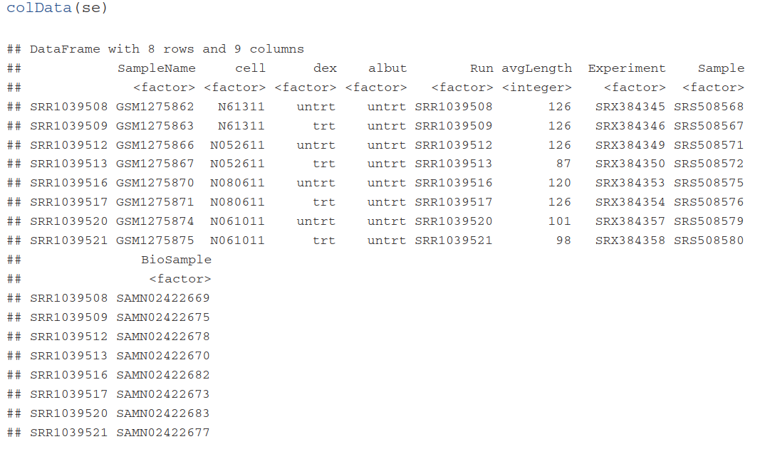
colData(se)         #查看sample信息，因为还没有制作所以目前是空的
(colData(se) <- DataFrame(sampleTable))  #将样本实验设计信息传递给colData(se)，文件3：colData信息。涉及到实验设计

-------------------------------------------------------------------------------------------------华丽丽的分割线----------------------------------------------------------------------

At this point, we have counted the fragments which overlap the genes in the gene model we specified。这里统计完之后，我们可以用一系列的包，进行差异分析，包括(limma,edgeR,DESeq2等)。下面我们将用DESeq2。在DESeq2中最主要的是构建 DESeqDataSet 对象，可以用上述 SummarizedExperiment objects转化为 DESeqDataSet objects。两者之间的区别是：

1）SummarizedExperiment 对象中的assay slot 被用 DESeq2中的counts accessor function代替, 且 DESeqDataSet class 强制表达矩阵中的values值为非负整数。

2）DESeqDataSet 包含design formula(设计公式)。实验设计在最初的分析中被指定，将 告诉DESeq2在分析中如何处理samples。

A second difference is that the DESeqDataSet has an associated design formula. The experimental design is specified at the beginning of the analysis, as it will inform many of the DESeq2 functions how to treat the samples in the analysis (one exception is the size factor estimation, i.e., the adjustment for differing library sizes, which does not depend on
the design formula). The design formula tells which columns in the sample information table (colData) specify the experimental design and how these factors should be used in the analysis

最简单的实验设计是 ~ condition，这里condition是 column in  colData(dds)，指定样本所在的分组。在airway experiment,这里我们指定实验设计为~ cell + dex表示希望检测对于不同cell line(cell). 进行dexamethasone controlling (dex，氟美松处理) 的效果。

----------------------------------------------------------------------------------------------------分割完毕-----------------------------------------------------------------------------

3、The DESeqDataSet, sample information, and the design formula

有两种方法构建 DESeqDataSet 对象：

3.1  Starting from SummarizedExperiment( 直接将SummarizedExperiment转化为DESeqDataSet )

以airway自带数据为例:

data("airway")
se <- airway
se$dex <- relevel(se$dex, "untrt")  #specify that untrt is the reference level for the dex variable
se$dex
round( colSums(assay(se)) / 1e6, 1 ) #count that uniquely aligned to the genes 。round表示四舍五入，1表示小数点后一位
colData(se)                #因为airway数据集制作好了这个矩阵，自己的数据需要用前面的方法制作这个。
library("DESeq2")
dds <- DESeqDataSet(se, design = ~ cell + dex)  #构建DESeqDataSet对象

3.2  Starting from  count matrices(  如果你之前没有准备SummarizedExperiment， 只有count matrix 和 sample information ，利用这两个文件及DESeqDataSetFromMatrix()函数构建 DESeqDataSet对象 )

countdata <- assay(se)   ##这里从前面的assay中取出表达矩阵用于演示，countdata: a table with the fragment counts
head(countdata, 3)
coldata <- colData(se)   ##这里从前面的assay中取出样本信息用于演示， coldata: a table with information about the samples
(ddsMat <- DESeqDataSetFromMatrix(countData = countdata,
                               colData = coldata,
                               design = ~ cell + dex)   #从countdata表达矩阵和coldata样本信息构建DESeqDataSet对象

4）Exploratory analysis and visualization(数据探索分析及可视化)

4.1 Pre-filtering the dataset

nrow(dds) #64102
dds <- dds[ rowSums(counts(dds)) > 1, ]#remove rows of the DESeqDataSet that have no counts, or only a single count across all samples:
nrow(dds)  #29391

4.2 The rlog transformation

需要rlog原因：

When the expected amount of variance is approximately the same across different mean values, the  data is said to be homoskedastic(同方差). For RRNA-seq raw counts, however, the variance grows with the mean. For example, if one performs PCA directly on a matrix of size-factor-normalized read counts, the result typically depends only on the few most strongly expressed genes because they show the largest absolute differences between samples. A simple  and often used strategy to avoid this is to take the logarithm of the normalized count values plus a small pseudocount; however, now the genes with the very lowest counts will tend to dominate the results because, due to the strong Poisson noise inherent to small count values, and the fact that the logarithm amplifies differences for the smallest values, these low count genes will show the strongest relative differences between samples.As a solution, DESeq2 offers transformations for count data that stabilize the variance across the mean. One such transformation is the regularized-logarithm transformation or rlog2. For genes with high counts, the rlog transformation will give similar result to the ordinary log2 transformation of normalized counts. For genes with lower counts, however, the values are shrunken towards the genes’ averages across all samples. Using an empirical Bayesian prior on inter-sample differences in the form of a ridge penalty, the rlog-transformed data then becomes approximately homoskedastic, and can be used directly for computing distances between samples and making PCA plots. Another transformation, the variance stabilizing transformation17, is discussed alongside the rlog in the DESeq2 vignette.

rlog()函数返回一个SummarizedExperiment对象，其中 assay slot包含 rlog-转换后的值。

rld <- rlog(dds, blind=FALSE)
head(assay(rld), 3)
par( mfrow = c( 1, 2 ) )
dds <- estimateSizeFactors(dds)  #估计size factors to account for sequencing depth
plot(log2(counts(dds, normalized=TRUE)[,1:2] + 1),pch=16, cex=0.3)  #then specify normalized=TRUE
plot(assay(rld)[,1:2],pch=16, cex=0.3)  #Sequencing depth correction is done automatically for the rlog method (and for varianceStabilizingTransformation).

普通的log2(左)及rlog2(右)之间的比较

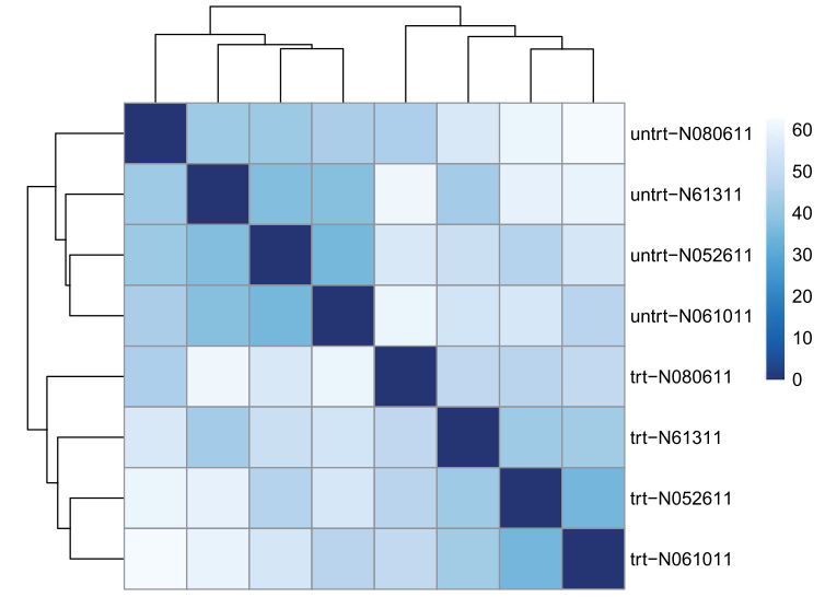
4.3 Sample distances

评估样本间关系(即总体相似度)，哪些样本更相近，哪些更远，是否符合实验设计？

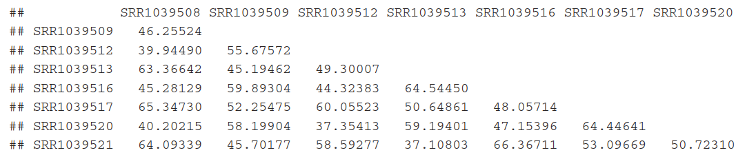
方法一：用欧式距离(Euclidean distance )，用rlog-transformed data(即normalized之后的矩阵)

sampleDists <- dist( t( assay(rld) ) )  #欧氏距离,为确保所有基因大致相同的contribution用rlog-transformed data
sampleDists

样本间关系，欧式距离。

library("pheatmap")      ##用热图展示样品间关系
library("RColorBrewer")
sampleDistMatrix <- as.matrix( sampleDists )
rownames(sampleDistMatrix) <- paste( rld$dex, rld$cell, sep="-" )
colnames(sampleDistMatrix) <- NULL
colors <- colorRampPalette( rev(brewer.pal(9, "Blues")) )(255)
pheatmap(sampleDistMatrix,
		clustering_distance_rows=sampleDists,
		clustering_distance_cols=sampleDists,
		col=colors)

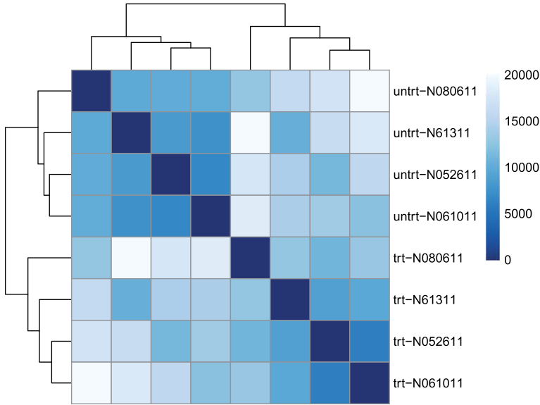
方法二：用 PoiClaClu 包计算泊松距离(Poisson Distance)，必须是原始表达矩阵。The PoissonDistance function takes the original count matrix
(not normalized) with samples as rows instead of columns, so we need to transpose the counts in dds.

library("PoiClaClu")
poisd <- PoissonDistance(t(counts(dds)))      ##对数据转置
samplePoisDistMatrix <- as.matrix( poisd$dd )  #计算样品间关系
rownames(samplePoisDistMatrix) <- paste( rld$dex, rld$cell, sep="-" )
colnames(samplePoisDistMatrix) <- NULL
pheatmap(samplePoisDistMatrix,
		clustering_distance_rows=poisd$dd,
		clustering_distance_cols=poisd$dd,
		col=colors)

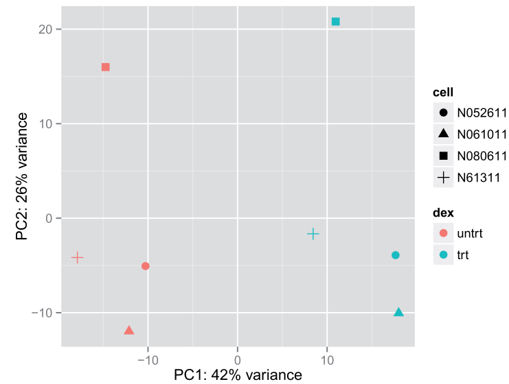
4.4 PCA plot(另一个展示样品间关系的图形)

一种方法是用DESeq2包中的plotPCA()函数

plotPCA(rld, intgroup = c("dex", "cell")) #DESeq2包plotPCA()函数

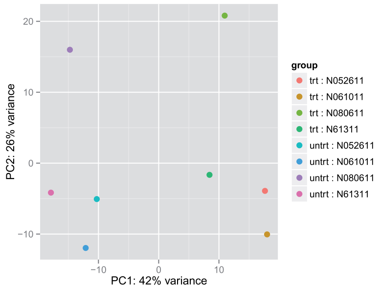
另一种方法是用ggplot2.需要调用 plotPCA()返回用于画图的数据

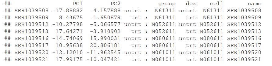
(data <- plotPCA(rld, intgroup = c( "dex", "cell"), returnData=TRUE))  #调用plotPCA生成要画图的data
percentVar <- round(100 * attr(data, "percentVar"))      #PC1,pC2
library("ggplot2")                                    #画图
ggplot(data, aes(PC1, PC2, color=dex, shape=cell)) + geom_point(size=3) +
 　　　　xlab(paste0("PC1: ",percentVar[1],"% variance")) +
　　 　　ylab(paste0("PC2: ",percentVar[2],"% variance"))

data:

4.4 MDS plot(另一种PCA图，multidimensional scaling (MDS) function )
在没有表达矩阵值，但只有一个距离矩阵的情况下使用。This is useful when we don’t have a matrix of data, but only a matrix of distances. Here we compute the MDS for the distances calculated from the rlog transformed counts and plot these。

##用归一化后的数据产生的距离矩阵(calculated from the rlog transformed)
mdsData <- data.frame(cmdscale(sampleDistMatrix))
mds <- cbind(mdsData, as.data.frame(colData(rld)))
ggplot(mds, aes(X1,X2,color=dex,shape=cell)) + geom_point(size=3)

###用原始数据产生的泊松距离矩阵(calculated from the raw)
mdsPoisData <- data.frame(cmdscale(samplePoisDistMatrix))
mdsPois <- cbind(mdsPoisData, as.data.frame(colData(dds)))
ggplot(mdsPois, aes(X1,X2,color=dex,shape=cell)) + geom_point(size=3)

5）Differential expression analysis（差异分析）

5,1）Running the differential expression pipeline

用DESeq()函数对原始表达矩阵进行差异表达分析(run the differential expression pipeline on the raw counts with a single call to the function DESeq)

dds <- DESeq(dds)  #差异表达分析

5.2）Building the results table

利用result函数()，将返回一个数据框对象,包含有 metadata information（每一列的意义）。

(res <- results(dds)) #产生log2 fold change 及p值
mcols(res, use.names=TRUE)  #查看meta信息
summary(res)  #产看其他信息

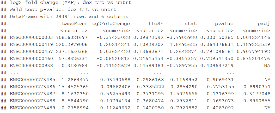
每列的含义：

baseMean：is a just the average of the normalized count values, dividing by size factors, taken over  all samples in the DESeqDataSet

log2FoldChange： the effect size estimate. It tells us how much the gene’s expression seems to  have changed due to treatment with dexamethasone in comparison to untreated samples

lfcSE：the standard error estimate for the log2 fold change estimate，(the effect size estimate has an uncertainty associated with it,)

p value:statistical test , the result of this test is reported as a p value. Remember that a p value indicates the probability that a fold change as strong as the observed one, or even stronger, would be seen under the situation described by the null hypothesis.

padj:adjusted p-value

2种更严格的方法去筛选显著差异基因：

降低false discovery rate threshold (the threshold on padj in the results table)
提升log2 fold change threshold(from 0 using the lfc Threshold argument of results)

#如果要降低false discovery rate threshold，将要设置的值传递给results(),使用该阈值进行独立的过滤：
res.05 <- results(dds, alpha=.05)  #设置阈值FDR=0.05
table(res.05$padj < .05)          #产看结果
#如果提升log2 fold change threshold show more substantial changes due to  treatment, we simply supply a value on the log2 scale.
resLFC1 <- results(dds, lfcThreshold=1)
table(resLFC1$padj < 0.1)

Sometimes a subset of the p values in res will be NA (“not available”). This is DESeq’s way of reporting that all counts for this gene were zero, and hence no test was applied. In addition, p values can be assigned NA if the gene was excluded from analysis because it contained an extreme count outlier. For more information, see the outlier detection  section of the DESeq2 vignette.

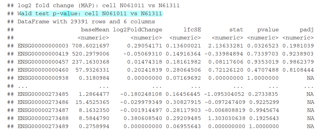
5.2）Other comparisons

可以利用result函数中的contrast参数来选择任何2组数据进行比较

results(dds, contrast=c("cell", "N061011", "N61311"))

5.3）Multiple testing（详细看文档理解FDR）

sum(res$pvalue < 0.05, na.rm=TRUE)
sum(!is.na(res$pvalue))
sum(res$padj < 0.1, na.rm=TRUE)
resSig <- subset(res, padj < 0.1)
head(resSig[ order(resSig$log2FoldChange), ])
head(resSig[ order(resSig$log2FoldChange, decreasing=TRUE), ])

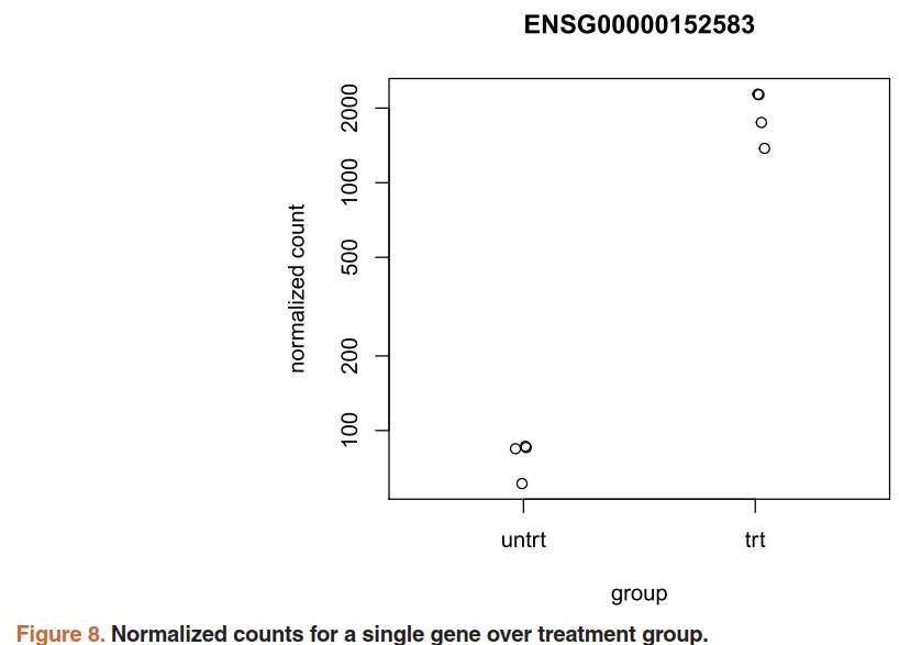
5.4）Plotting results

用 plotCounts()函数查看特定基因的表达量：需要三个参数，DESeqDataSet, gene name, and the group over which to plot the counts (Figure 8).

topGene <- rownames(res)[which.min(res$padj)]
plotCounts(dds, gene=topGene, intgroup=c("dex"))

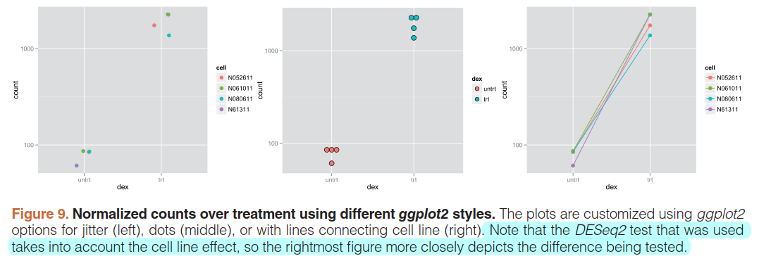
也可以用ggplot2画传统的散点图

data <- plotCounts(dds, gene=topGene, intgroup=c("dex","cell"), returnData=TRUE)
ggplot(data, aes(x=dex, y=count, color=cell)) +
 scale_y_log10() +
 geom_point(position=position_jitter(width=.1,height=0), size=3)

ggplot(data, aes(x=dex, y=count, fill=dex)) +
 scale_y_log10() +
 geom_dotplot(binaxis="y", stackdir="center")

ggplot(data, aes(x=dex, y=count, color=cell, group=cell)) +
 scale_y_log10() + geom_point(size=3) + geom_line()

An MA-plot provides a useful overview for an experiment with a two-group comparison：

plotMA(res, ylim=c(-5,5))

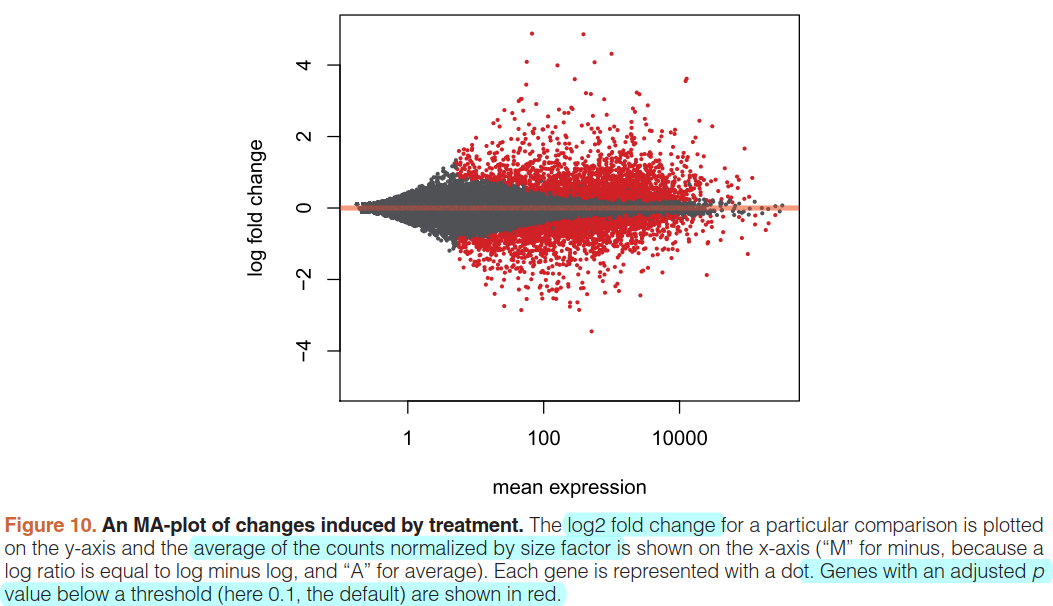
可以看到DESeq通过统计学技术，narrowing垂直方向的离散(左部分)

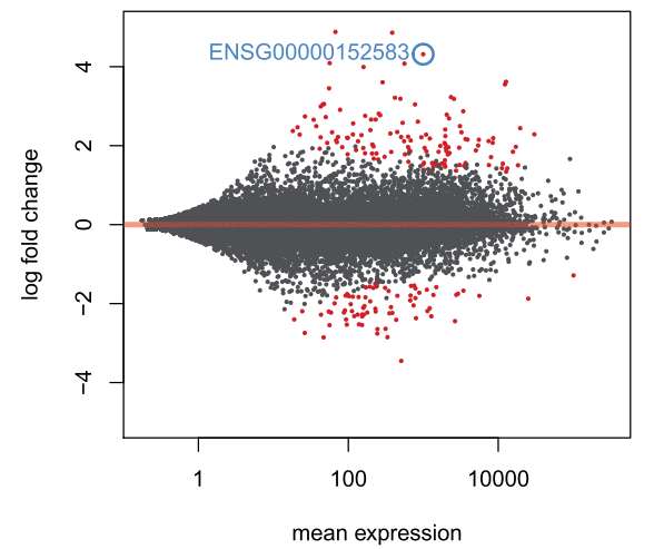
make an MA-plot for the results table in which we raised the log2 fold change threshold，并标记除特定的一个基因：

plotMA(resLFC1, ylim=c(-5,5))
topGene <- rownames(resLFC1)[which.min(resLFC1$padj)]
with(resLFC1[topGene, ], {
 points(baseMean, log2FoldChange, col="dodgerblue", cex=2, lwd=2)
 text(baseMean, log2FoldChange, topGene, pos=2, col="dodgerblue")
})

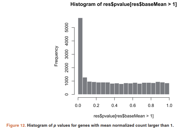
histogram of the p values：

hist(res$pvalue[res$baseMean > 1], breaks=0:20/20, col="grey50", border="white")

5.5）Plotting results

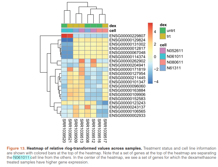
提取前20个highest variance across samples.基因进行聚类

library("genefilter")
topVarGenes <- head(order(rowVars(assay(rld)),decreasing=TRUE),20)
mat <- assay(rld)[ topVarGenes, ]
mat <- mat - rowMeans(mat)
df <- as.data.frame(colData(rld)[,c("cell","dex")])
pheatmap(mat, annotation_col=df)

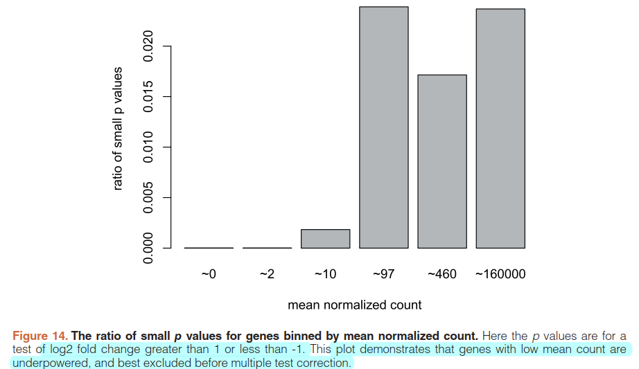
5.6）Independent filtering

qs <- c(0, quantile(resLFC1$baseMean[resLFC1$baseMean > 0], 0:6/6))
bins <- cut(resLFC1$baseMean, qs)
levels(bins) <- paste0("~",round(signif(.5*qs[-1] + .5*qs[-length(qs)],2)))
ratios <- tapply(resLFC1$pvalue, bins, function(p) mean(p < .05, na.rm=TRUE))
barplot(ratios, xlab="mean normalized count", ylab="ratio of small p values")

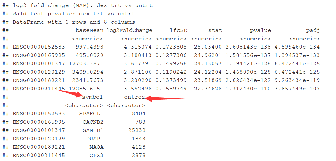
5.7）Annotating and exporting results

因为这里只有Ensembl gene IDs，而其它的名称也非常有用。用 mapIds()函数, 其中column 参数表示需要哪种信息， multiVals参数表示如果有多个对应值的时候如何选择.，这里选择第一个. 调用两次函数 add the gene symbol  and Entrez ID.

library("AnnotationDbi")
library("org.Hs.eg.db")
columns(org.Hs.eg.db)
res$symbol <- mapIds(org.Hs.eg.db,
		　　keys=row.names(res),
		　　column="SYMBOL", #需要哪种信息
		　　keytype="ENSEMBL",
		　　multiVals="first") #有多个对应值，这里选第一个
res$entrez <- mapIds(org.Hs.eg.db,
		keys=row.names(res),
		column="ENTREZID",
		keytype="ENSEMBL",
	　　　　　multiVals="first")
resOrdered <- res[order(res$padj),]
head(resOrdered)

5.8）Annotating and exporting results

resOrderedDF <- as.data.frame(resOrdered)[1:100,]
write.csv(resOrderedDF, file="results.csv")    #保存结果

library("ReportingTools")                     #生成网页版结果
htmlRep <- HTMLReport(shortName="report", title="My report",
 reportDirectory="./report")
publish(resOrderedDF, htmlRep)
url <- finish(htmlRep)
browseURL(url)

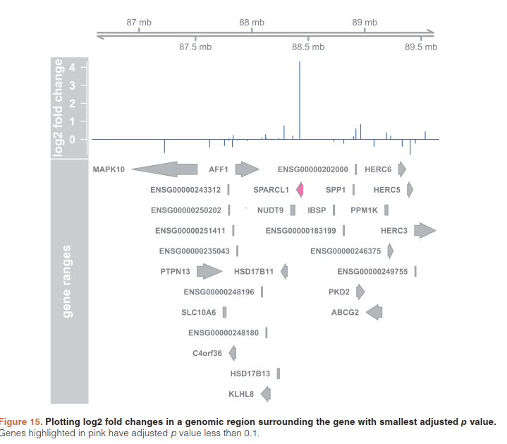
5.9）Plotting fold changes in genomic space

在基因组上展示差异结果

(resGR <- results(dds, lfcThreshold=1, format="GRanges"))
resGR$symbol <- mapIds(org.Hs.eg.db, names(resGR), "SYMBOL", "ENSEMBL")  #加基因名
library("Gviz")  #用于可视化for plotting the GRanges and associated metadata: the log fold changes due to dexam- ethasone treatment.
window <- resGR[topGene] + 1e6
strand(window) <- "*"
resGRsub <- resGR[resGR %over% window]
naOrDup <- is.na(resGRsub$symbol) | duplicated(resGRsub$symbol)
resGRsub$group <- ifelse(naOrDup, names(resGRsub), resGRsub$symbol)

sig <- factor(ifelse(resGRsub$padj < .1 & !is.na(resGRsub$padj),"sig","notsig"))
options(ucscChromosomeNames=FALSE)
g <- GenomeAxisTrack()
a <- AnnotationTrack(resGRsub, name="gene ranges", feature=sig)
d <- DataTrack(resGRsub, data="log2FoldChange", baseline=0,
 type="h", name="log2 fold change", strand="+")
plotTracks(list(g,d,a), groupAnnotation="group", notsig="grey", sig="hotpink")

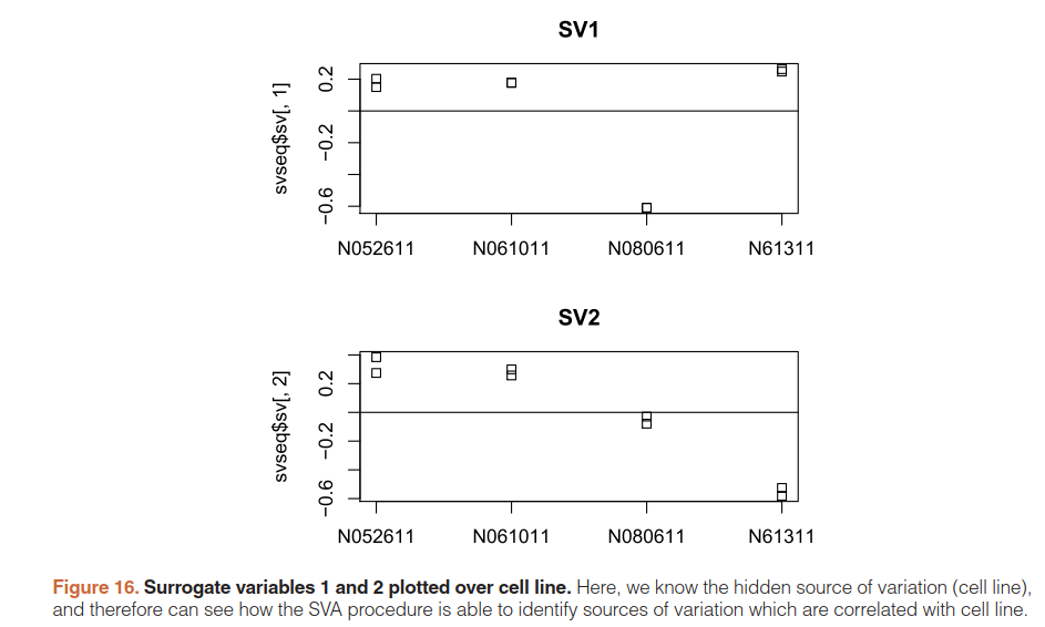
5.10）Removing hidden batch effects

详细看文档

library("sva")
dat <- counts(dds, normalized=TRUE)
idx <- rowMeans(dat) > 1
dat <- dat[idx,]
mod <- model.matrix(~ dex, colData(dds))
mod0 <- model.matrix(~ 1, colData(dds))
svseq <- svaseq(dat, mod, mod0, n.sv=2)
svseq$sv
par(mfrow=c(2,1),mar=c(3,5,3,1))
stripchart(svseq$sv[,1] ~ dds$cell,vertical=TRUE,main="SV1")
abline(h=0)
stripchart(svseq$sv[,2] ~ dds$cell,vertical=TRUE,main="SV2")
abline(h=0)
ddssva <- dds
ddssva$SV1 <- svseq$sv[,1]
ddssva$SV2 <- svseq$sv[,2]
design(ddssva) <- ~ SV1 + SV2 + dex
ddssva <- DESeq(ddssva)

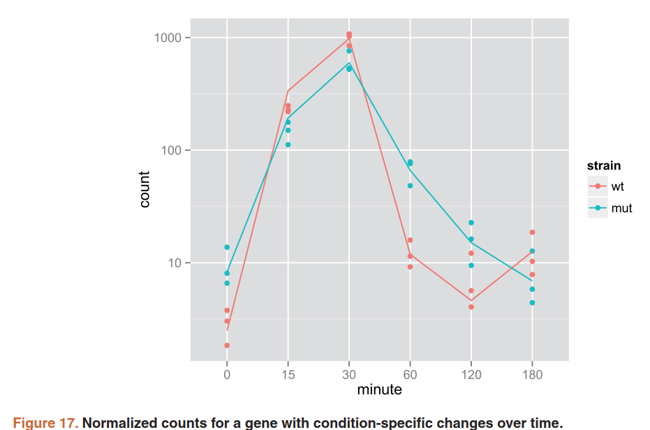
5.11）Time course experiments

详细看文档

library("fission")
data("fission")
ddsTC <- DESeqDataSet(fission, ~ strain + minute + strain:minute)
ddsTC <- DESeq(ddsTC, test="LRT", reduced = ~ strain + minute)
resTC <- results(ddsTC)
resTC$symbol <- mcols(ddsTC)$symbol
head(resTC[order(resTC$padj),],4)
data <- plotCounts(ddsTC, which.min(resTC$padj),
intgroup=c("minute","strain"), returnData=TRUE)
ggplot(data, aes(x=minute, y=count, color=strain, group=strain)) +
　　　　 geom_point() + stat_smooth(se=FALSE,method="loess") + scale_y_log10()
resultsNames(ddsTC)
res30 <- results(ddsTC, name="strainmut.minute30", test="Wald")
res30[which.min(resTC$padj),]

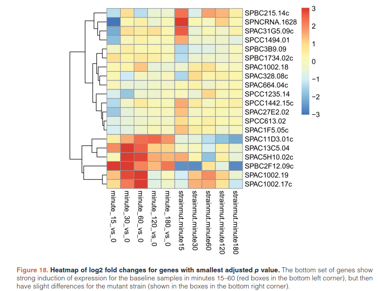
furthermore cluster significant genes by their profiles：

betas <- coef(ddsTC)
colnames(betas)
library("pheatmap")
topGenes <- head(order(resTC$padj),20)
mat <- betas[topGenes, -c(1,2)]
thr <- 3
mat[mat < -thr] <- -thr
mat[mat > thr] <- thr
pheatmap(mat, breaks=seq(from=-thr, to=thr, length=101),
		cluster_col=FALSE)