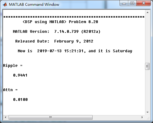
《DSP using MATLAB》Problem 8.28

代码：

%% ------------------------------------------------------------------------
%%            Output Info about this m-file
fprintf('\n***********************************************************\n');
fprintf('        <DSP using MATLAB> Problem 8.28 \n\n');

banner();
%% ------------------------------------------------------------------------

Fp =  500;                    % analog passband freq in Hz
Fs =  700;                    % analog stopband freq in Hz
fs = 2000;                    % sampling rate in Hz

% -------------------------------
%       ω = ΩT = 2πF/fs
% Digital Filter Specifications:
% -------------------------------
wp = 2*pi*Fp/fs;                 % digital passband freq in rad/sec
%wp = Fp;
ws = 2*pi*Fs/fs;                 % digital stopband freq in rad/sec
%ws = Fs;
Rp = 0.5;                        % passband ripple in dB
As = 40;                         % stopband attenuation in dB

Ripple = 10 ^ (-Rp/20)           % passband ripple in absolute
Attn = 10 ^ (-As/20)             % stopband attenuation in absolute

% Analog prototype specifications: Inverse Mapping for frequencies
T = 1/fs;                       % set T = 1
OmegaP = wp/T;               % prototype passband freq
OmegaS = ws/T;               % prototype stopband freq

% Analog Chebyshev-1 Prototype Filter Calculation:
[cs, ds] = afd_chb1(OmegaP, OmegaS, Rp, As);

% Calculation of second-order sections:
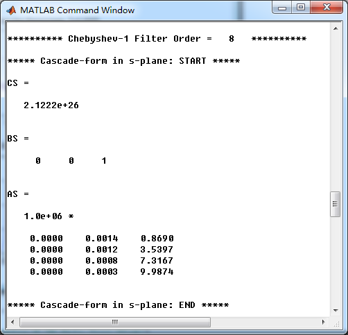
fprintf('\n***** Cascade-form in s-plane: START *****\n');
[CS, BS, AS] = sdir2cas(cs, ds)
fprintf('\n***** Cascade-form in s-plane: END *****\n');

% Calculation of Frequency Response:
[db_s, mag_s, pha_s, ww_s] = freqs_m(cs, ds, 2*pi/T);

% Calculation of Impulse Response:
[ha, x, t] = impulse(cs, ds);

% Match-z Transformation:
%[b, a] = imp_invr(cs, ds, T)        % digital Num and Deno coefficients of H(z)
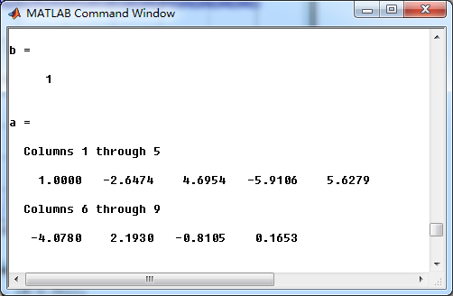
[b, a] = mzt(cs, ds, T)            % digital Num and Deno coefficients of H(z)
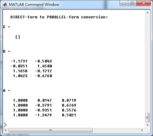
[C, B, A] = dir2par(b, a)

% Calculation of Frequency Response:
[db, mag, pha, grd, ww] = freqz_m(b, a);

%% -----------------------------------------------------------------
%%                             Plot
%% -----------------------------------------------------------------
figure('NumberTitle', 'off', 'Name', 'Problem 8.28 Analog Chebyshev-1 lowpass')
set(gcf,'Color','white');
M = 1.2;                          % Omega max

subplot(2,2,1); plot(ww_s/(pi*1000), mag_s);  grid on; axis([-1.5, 1.5, 0, 1.1]);
xlabel(' Analog frequency in k\pi units'); ylabel('|H|'); title('Magnitude in Absolute');
set(gca, 'XTickMode', 'manual', 'XTick', [-700, -500, 0, 500, 700, 1000]*0.002);
set(gca, 'YTickMode', 'manual', 'YTick', [0, 0.01, 0.5, 0.9441, 1]);

subplot(2,2,2); plot(ww_s/(pi*1000), db_s);  grid on; %axis([0, M, -50, 10]);
xlabel('Analog frequency in k\pi units'); ylabel('Decibels'); title('Magnitude in dB ');
set(gca, 'XTickMode', 'manual', 'XTick', [-700, -500, 0, 500, 700, 1000]*0.002);
set(gca, 'YTickMode', 'manual', 'YTick', [-70, -40, -1, 0]);
set(gca,'YTickLabelMode','manual','YTickLabel',['70';'40';' 1';' 0']);

subplot(2,2,3); plot(ww_s/(pi*1000), pha_s/pi);  grid on; axis([-1.5, 1.5, -1.2, 1.2]);
xlabel('Analog frequency in k\pi nuits'); ylabel('radians'); title('Phase Response');
set(gca, 'XTickMode', 'manual', 'XTick', [-700, -500, 0, 500, 700, 1000]*0.002);
set(gca, 'YTickMode', 'manual', 'YTick', [-1:0.5:1]);

subplot(2,2,4); plot(t, ha); grid on; %axis([0, 30, -0.05, 0.25]);
xlabel('time in seconds'); ylabel('ha(t)'); title('Impulse Response');

figure('NumberTitle', 'off', 'Name', 'Problem 8.28 Digital Chebyshev-1 lowpass')
set(gcf,'Color','white');
M = 2;                          % Omega max

%%  Note  %%
%%  Magnitude of H(z) * T
%%  Note  %%
subplot(2,2,1); plot(ww/pi, mag/10);  grid on; axis([0, M, 0, 1.1]);
xlabel(' frequency in \pi units'); ylabel('|H|'); title('Magnitude Response');
set(gca, 'XTickMode', 'manual', 'XTick', [0, 0.5, 0.7, 1.0, M]);
set(gca, 'YTickMode', 'manual', 'YTick', [0, 0.01, 0.5, 0.9441, 1, 5, 10]);

subplot(2,2,2); plot(ww/pi, pha/pi); axis([0, M, -1.1, 1.1]); grid on;
xlabel('frequency in \pi nuits'); ylabel('radians in \pi units'); title('Phase Response');
set(gca, 'XTickMode', 'manual', 'XTick', [0, 0.5, 0.7, 1.0, M]);
set(gca, 'YTickMode', 'manual', 'YTick', [-1:1:1]);

subplot(2,2,3); plot(ww/pi, db); axis([0, M, -70, 10]); grid on;
xlabel('frequency in \pi units'); ylabel('Decibels'); title('Magnitude in dB ');
set(gca, 'XTickMode', 'manual', 'XTick', [0, 0.5, 0.7, 1.0, M]);
set(gca, 'YTickMode', 'manual', 'YTick', [-50, -40, -1, 0]);
set(gca,'YTickLabelMode','manual','YTickLabel',['50';'40';' 1';' 0']);

subplot(2,2,4); plot(ww/pi, grd); grid on; %axis([0, M, 0, 35]);
xlabel('frequency in \pi units'); ylabel('Samples'); title('Group Delay');
set(gca, 'XTickMode', 'manual', 'XTick', [0, 0.5, 0.7, 1.0, M]);
%set(gca, 'YTickMode', 'manual', 'YTick', [0:5:35]);

figure('NumberTitle', 'off', 'Name', 'Problem 8.28 Pole-Zero Plot')
set(gcf,'Color','white');
zplane(b,a);
title(sprintf('Pole-Zero Plot'));
%pzplotz(b,a);

% Calculation of Impulse Response:
%[hs, xs, ts] = impulse(c, d);
figure('NumberTitle', 'off', 'Name', 'Problem 8.28 Imp & Freq Response')
set(gcf,'Color','white');
t = [0:0.0005:0.04]; subplot(2,1,1); impulse(cs,ds,t); grid on;   % Impulse response of the analog filter
axis([0, 0.04, -500, 1000]);hold on

n = [0:1:0.04/T]; hn = filter(b,a,impseq(0,0,0.04/T));             % Impulse response of the digital filter
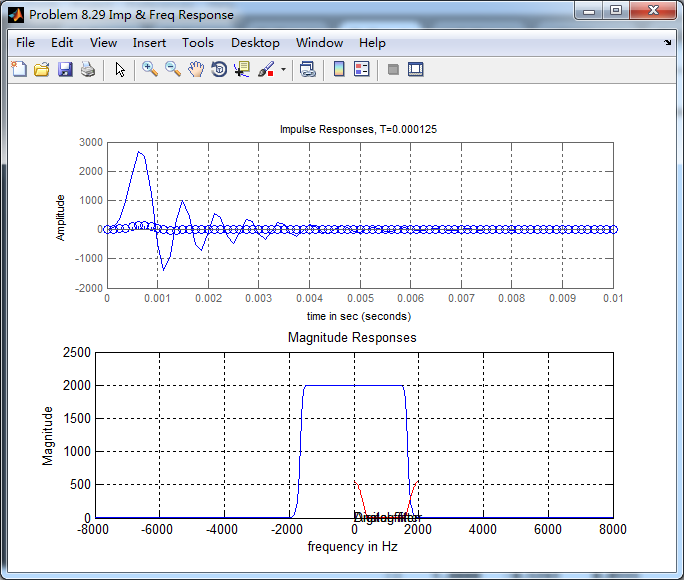
stem(n*T,hn); xlabel('time in sec'); title (sprintf('Impulse Responses, T=%.4f',T));
hold off

%n = [0:1:29];
%hz = impz(b, a, n);

% Calculation of Frequency Response:
[dbs, mags, phas, wws] = freqs_m(cs, ds, 2*pi/T);             % Analog frequency   s-domain  

[dbz, magz, phaz, grdz, wwz] = freqz_m(b, a);                 % Digital  z-domain

%% -----------------------------------------------------------------
%%                             Plot
%% -----------------------------------------------------------------  

M = 1/T;                          % Omega max

subplot(2,1,2); plot(wws/(2*pi),mags*Fs,'b', wwz/(2*pi)*Fs,magz,'r'); grid on;

xlabel('frequency in Hz'); title('Magnitude Responses'); ylabel('Magnitude'); 

text(1.4,.5,'Analog filter'); text(1.5,1.5,'Digital filter');

　　运行结果：

转换成绝对指标

模拟Chebyshev-1型低通滤波器，系统函数串联形式

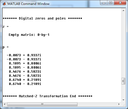
通过match-z方法，模拟低通转换成数字Chebyshev-1型低通滤波器，

数字Chebyshev-1型低通直接形式的系数

转换成并联形式，其系数

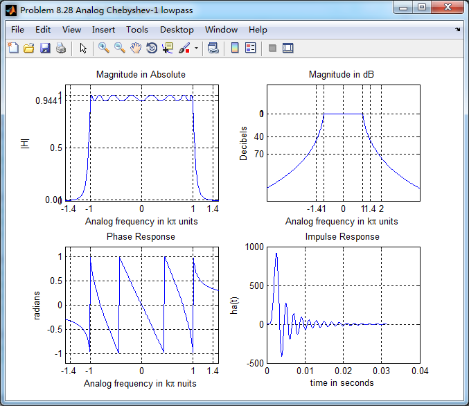
模拟低通的幅度谱、相位谱和脉冲响应

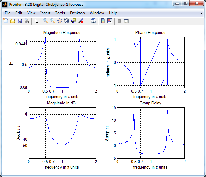
数字低通的幅度谱、相位谱和群延迟

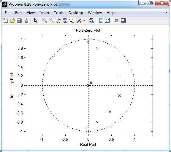
数字低通的零极点图，可以看出，零极点都位于单位圆内。

match-z方法，是和脉冲响应不变法不同的，不保留脉冲响应的形式，模拟Chebyshev-1型低通滤波器和对应的数字低通

滤波器的脉冲响应形式是不同的，见下图。