实现一个单隐层神经网络python

　　仅仅记录神经网络编程主线。

一引用工具包

import numpy as np

import matplotlib.pyplot as plt

from testCases import *

import sklearn

import sklearn.datasets

import sklearn.linear_model

from planar_utils import plot_decision_boundary, sigmoid, load_planar_dataset, load_extra_datasets

%matplotlib inline

np.random.seed() # set a seed so that the results are consistent

　　二读入数据集

　　输入函数实现在最下面附录

X, Y = load_planar_dataset()

　　lanar是二分类数据集，可视化如下图，外形像花的一样的非线性数据集。

plt.scatter(X[, :], X[, :], c=Y, s=, cmap=plt.cm.Spectral);

- 特征 (x1, x2)

- 类别 (red:0, blue:1).

三神经网络结构

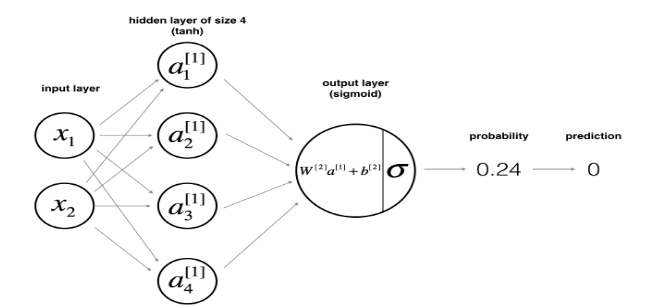
　对于输入样本x，前向传播计算如下公式：

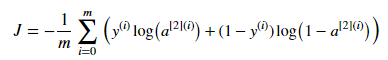
损失函数J：

输入样本X：[n_x,m]; 假设输入m个样本，每个样本k维，输入神经元n_x个数=特征维度k，输出神经个数n_y=类别个数。

W1:[n_h,n_x];
b1:[n_h,1];
W2:[n_y,n_h];
b2:[n_y,1];
trick：Wi第一维是第i+1层的神经元个数，第二维是第i层的神经元个数；bi第一维是第i层的神经元个数，第二维永远是1，因为python有broadcast机制，自动对齐。

def layer_sizes(X, Y):
"""
Arguments:
X -- input dataset of shape (input size, number of examples)
Y -- labels of shape (output size, number of examples)

Returns:
n_x -- the size of the input layer
n_h -- the size of the hidden layer
n_y -- the size of the output layer
"""
### START CODE HERE ### (≈ 3 lines of code)
n_x = X.shape[0] # size of input layer
n_h = 4
n_y = Y.shape[0] # size of output layer
### END CODE HERE ###
return (n_x, n_h, n_y)

四初始化参数

　W1，W2：不能初始化为0矩阵，如果这样第一个隐藏所有神经元梯度都和第一个一样: np.random.randn(a,b) * 0.01 .

b1，b2.：初始化为0向量 np.zeros((a,b)).

def initialize_parameters(n_x, n_h, n_y):
"""
Argument:
n_x -- size of the input layer
n_h -- size of the hidden layer
n_y -- size of the output layer

Returns:
params -- python dictionary containing your parameters:
W1 -- weight matrix of shape (n_h, n_x)
b1 -- bias vector of shape (n_h, 1)
W2 -- weight matrix of shape (n_y, n_h)
b2 -- bias vector of shape (n_y, 1)
"""

np.random.seed(2) # we set up a seed so that your output matches ours although the initialization is random.

### START CODE HERE ### (≈ 4 lines of code)
W1 = np.random.randn(n_h, n_x)*0.01
b1 = np.zeros((n_h, 1))
W2 = np.random.randn(n_y, n_h)*0.01
b2 = np.zeros((n_y, 1))
### END CODE HERE ###

assert (W1.shape == (n_h, n_x))
assert (b1.shape == (n_h, 1))
assert (W2.shape == (n_y, n_h))
assert (b2.shape == (n_y, 1))

parameters = {"W1": W1,
"b1": b1,
"W2": W2,
"b2": b2}

return parameters

五前向传播

　　cache缓存计算结果，反向传播需要。

def forward_propagation(X, parameters):
"""
Argument:
X -- input data of size (n_x, m)
parameters -- python dictionary containing your parameters (output of initialization function)

Returns:
A2 -- The sigmoid output of the second activation
cache -- a dictionary containing "Z1", "A1", "Z2" and "A2"
"""
# Retrieve each parameter from the dictionary "parameters"
### START CODE HERE ### (≈ 4 lines of code)
W1 = parameters['W1']
b1 = parameters['b1']
W2 = parameters['W2']
b2 = parameters['b2']
### END CODE HERE ###

# Implement Forward Propagation to calculate A2 (probabilities)
### START CODE HERE ### (≈ 4 lines of code)
Z1 = np.dot(W1, X) + b1
A1 = np.tanh(Z1)
Z2 = np.dot(W2, A1) + b2
A2 = sigmoid(Z2)
### END CODE HERE ###

assert(A2.shape == (1, X.shape[1]))

cache = {"Z1": Z1,
"A1": A1,
"Z2": Z2,
"A2": A2}

return A2, cache

六计算损失函数

def compute_cost(A2, Y, parameters):
"""
Computes the cross-entropy cost given in equation (13)

Arguments:
A2 -- The sigmoid output of the second activation, of shape (1, number of examples)
Y -- "true" labels vector of shape (1, number of examples)
parameters -- python dictionary containing your parameters W1, b1, W2 and b2

Returns:
cost -- cross-entropy cost given equation (13)
"""

m = float(Y.shape[1]) # number of example

# Compute the cross-entropy cost
### START CODE HERE ### (≈ 2 lines of code)
logprobs = np.multiply(np.log(A2),Y) + np.multiply((1-Y), (np.log(1-A2)))
cost = -1/m * np.sum(logprobs)
### END CODE HERE ###

cost = np.squeeze(cost) # makes sure cost is the dimension we expect.
# E.g., turns [[17]] into 17
assert(isinstance(cost, float))

return cost

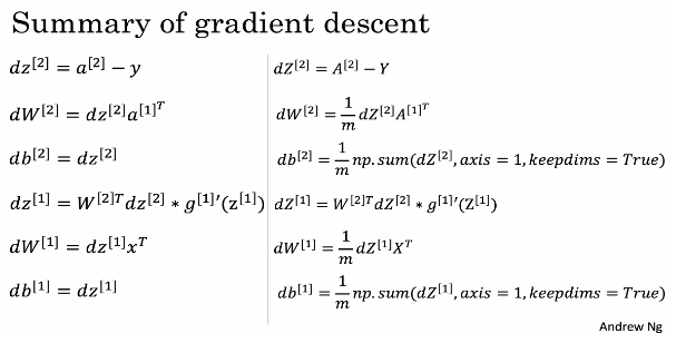
七反向传播

每个参数的维度
- dW1:[n_h,n_x];
- db1:[n_h,1];
- dW2:[n_y,n_h];
- db2:[n_y,1];
trick：dW1,db1,dW2,db2和W1,b1,W2,b2的维度一模一样。

def backward_propagation(parameters, cache, X, Y):
"""
Implement the backward propagation using the instructions above.

Arguments:
parameters -- python dictionary containing our parameters
cache -- a dictionary containing "Z1", "A1", "Z2" and "A2".
X -- input data of shape (2, number of examples)
Y -- "true" labels vector of shape (1, number of examples)

Returns:
grads -- python dictionary containing your gradients with respect to different parameters
"""
m = float(X.shape[1])

# First, retrieve W1 and W2 from the dictionary "parameters".
### START CODE HERE ### (≈ 2 lines of code)
W1 = parameters['W1']
W2 = parameters['W2']
### END CODE HERE ###

# Retrieve also A1 and A2 from dictionary "cache".
### START CODE HERE ### (≈ 2 lines of code)
A1 = cache['A1']
A2 = cache['A2']
### END CODE HERE ###

# Backward propagation: calculate dW1, db1, dW2, db2.
### START CODE HERE ### (≈ 6 lines of code, corresponding to 6 equations on slide above)
dZ2= A2 - Y
dW2 =1/m * np.dot(dZ2, A1.T)
db2 =1/m * np.sum(dZ2, axis=1, keepdims=True)
dZ1 = np.dot(W2.T, dZ2) * (1 - np.power(A1, 2))
dW1 = 1/m * np.dot(dZ1, X.T)
db1 =1/m * np.sum(dZ1, axis=1, keepdims=True)
### END CODE HERE ###

grads = {"dW1": dW1,
"db1": db1,
"dW2": dW2,
"db2": db2}

return grads

八梯度更新　

优化过程，梯度更新: 使用 (dW1, db1, dW2, db2) 更新参数 (W1, b1, W2, b2).

梯度下降公式: 其中 α 是学习率.

学习率: 如图所示，不同学习率，熟练情况不一样.

def update_parameters(parameters, grads, learning_rate = 1.2):
"""
Updates parameters using the gradient descent update rule given above

Arguments:
parameters -- python dictionary containing your parameters
grads -- python dictionary containing your gradients

Returns:
parameters -- python dictionary containing your updated parameters
"""
# Retrieve each parameter from the dictionary "parameters"
### START CODE HERE ### (≈ 4 lines of code)
W1 = parameters['W1']
b1 = parameters['b1']
W2 = parameters['W2']
b2 = parameters['b2']
### END CODE HERE ###

# Retrieve each gradient from the dictionary "grads"
### START CODE HERE ### (≈ 4 lines of code)
dW1 = grads["dW1"]
db1 = grads["db1"]
dW2 = grads["dW2"]
db2 = grads["db2"]
## END CODE HERE ###

# Update rule for each parameter
### START CODE HERE ### (≈ 4 lines of code)
W1 = W1 - learning_rate * dW1
b1 = b1 - learning_rate * db1
W2 = W2 - learning_rate * dW2
b2 = b2 - learning_rate * db2
### END CODE HERE ###

parameters = {"W1": W1,
"b1": b1,
"W2": W2,
"b2": b2}

return parameters

九模型　

将前面的函数整合成模型：

　　实现步骤:

1. 定义网络结构.

2. 初始化参数

3. Loop:

    - 前向传播

    - 计算损失函数

    - 反向传播计算梯度

    - 更新梯度

def nn_model(X, Y, n_h, num_iterations = 10000, print_cost=False):
"""
Arguments:
X -- dataset of shape (2, number of examples)
Y -- labels of shape (1, number of examples)
n_h -- size of the hidden layer
num_iterations -- Number of iterations in gradient descent loop
print_cost -- if True, print the cost every 1000 iterations

Returns:
parameters -- parameters learnt by the model. They can then be used to predict.
"""

np.random.seed(3)
n_x = layer_sizes(X, Y)[0]
n_y = layer_sizes(X, Y)[2]

# Initialize parameters, then retrieve W1, b1, W2, b2. Inputs: "n_x, n_h, n_y". Outputs = "W1, b1, W2, b2, parameters".
### START CODE HERE ### (≈ 5 lines of code)
n_x, n_h, n_y = layer_sizes(X, Y)
parameters = initialize_parameters(n_x, n_h, n_y)
W1 = parameters['W1']
b1 = parameters['b1']
W2 = parameters['W2']
b2 = parameters['b2']
### END CODE HERE ###

# Loop (gradient descent)

for i in range(0, num_iterations):

### START CODE HERE ### (≈ 4 lines of code)
# Forward propagation. Inputs: "X, parameters". Outputs: "A2, cache".
A2, cache = forward_propagation(X, parameters)

# Cost function. Inputs: "A2, Y, parameters". Outputs: "cost".
cost = compute_cost(A2, Y, parameters)

# Backpropagation. Inputs: "parameters, cache, X, Y". Outputs: "grads".
grads = backward_propagation(parameters, cache, X, Y)

# Gradient descent parameter update. Inputs: "parameters, grads". Outputs: "parameters".
parameters = update_parameters(parameters, grads)

### END CODE HERE ###

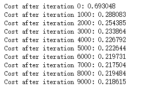
# Print the cost every 1000 iterations
if print_cost and i % 1000 == 0:
print ("Cost after iteration %i: %f" %(i, cost))

return parameters

十预测　

对于一个样本，预估概率大于阈值0.5的为1，否则为0.

def predict(parameters, X):
"""
Using the learned parameters, predicts a class for each example in X

Arguments:
parameters -- python dictionary containing your parameters
X -- input data of size (n_x, m)

Returns
predictions -- vector of predictions of our model (red: 0 / blue: 1)
"""

# Computes probabilities using forward propagation, and classifies to 0/1 using 0.5 as the threshold.
### START CODE HERE ### (≈ 2 lines of code)
A2, cache = forward_propagation(X, parameters)
predictions = np.array( [1 if x >0.5 else 0 for x in A2.reshape(-1,1)] ).reshape(A2.shape) # 这一行代码的作用详见下面代码示例
### END CODE HERE ###

return predictions

planar数据集测试单隐层神经网络性能，隐层神经元个数设置为4.

# Build a model with a n_h-dimensional hidden layer

parameters = nn_model(X, Y, n_h = , num_iterations = , print_cost=True)

# Plot the decision boundary

plot_decision_boundary(lambda x: predict(parameters, x.T), X, Y)

plt.title("Decision Boundary for hidden layer size " + str())

输出结果

附录：load输入数据集

import matplotlib.pyplot as plt

import numpy as np

import sklearn

import sklearn.datasets

import sklearn.linear_model

def plot_decision_boundary(model, X, y):

    # Set min and max values and give it some padding

    x_min, x_max = X[, :].min() - , X[, :].max() +

    y_min, y_max = X[, :].min() - , X[, :].max() +

    h = 0.01

    # Generate a grid of points with distance h between them

    xx, yy = np.meshgrid(np.arange(x_min, x_max, h), np.arange(y_min, y_max, h))

    # Predict the function value for the whole grid

    Z = model(np.c_[xx.ravel(), yy.ravel()])

    Z = Z.reshape(xx.shape)

    # Plot the contour and training examples

    plt.contourf(xx, yy, Z, cmap=plt.cm.Spectral)

    plt.ylabel('x2')

    plt.xlabel('x1')

    plt.scatter(X[, :], X[, :], c=y, cmap=plt.cm.Spectral)

def sigmoid(x):

    """

    Compute the sigmoid of x

    Arguments:

    x -- A scalar or numpy array of any size.

    Return:

    s -- sigmoid(x)

    """

    s = /(+np.exp(-x))

    return s

def load_planar_dataset():

    np.random.seed()

    m =  # number of examples

    N = int(m/) # number of points per class

    D =  # dimensionality

    X = np.zeros((m,D)) # data matrix where each row is a single example

    Y = np.zeros((m,), dtype='uint8') # labels vector ( for red,  for blue)

    a =  # maximum ray of the flower

    for j in range():

        ix = range(N*j,N*(j+))

        t = np.linspace(j*3.12,(j+)*3.12,N) + np.random.randn(N)*0.2 # theta

        r = a*np.sin(*t) + np.random.randn(N)*0.2 # radius

        X[ix] = np.c_[r*np.sin(t), r*np.cos(t)]

        Y[ix] = j

    X = X.T

    Y = Y.T

    return X, Y

def load_extra_datasets():

    N =

    noisy_circles = sklearn.datasets.make_circles(n_samples=N, factor=., noise=.)

    noisy_moons = sklearn.datasets.make_moons(n_samples=N, noise=.)

    blobs = sklearn.datasets.make_blobs(n_samples=N, random_state=, n_features=, centers=)

    gaussian_quantiles = sklearn.datasets.make_gaussian_quantiles(mean=None, cov=0.5, n_samples=N, n_features=, n_classes=, shuffle=True, random_state=None)

    no_structure = np.random.rand(N, ), np.random.rand(N, )

    return noisy_circles, noisy_moons, blobs, gaussian_quantiles, no_structure

参考: