[IR] Word Embeddings

In this tutorial we look at the word2vec model by Mikolov et al. This model is used for learning vector representations of words, called "word embeddings".

Highlights

This tutorial is meant to highlight the interesting, substantive parts of building a word2vec model in TensorFlow.

We start by giving the motivation for why we would want to represent words as vectors.
We look at the intuition behind the model and how it is trained (with a splash of math for good measure).
We also show a simple implementation of the model in TensorFlow.
Finally, we look at ways to make the naive version scale better.

tensorflow/examples/tutorials/word2vec/word2vec_basic.py

This basic example contains the code needed to download some data, train on it a bit and visualize the result.

Once you get comfortable with reading and running the basic version, you can graduate to models/tutorials/embedding/word2vec.py

which is a more serious implementation that showcases some more advanced TensorFlow principles about how to efficiently use threads to move data into a text model, how to checkpoint during training, etc.

Motivation: Why Learn Word Embeddings?

However, natural language processing systems traditionally treat words as discrete atomic symbols, and therefore 'cat' may be represented as Id537 and 'dog' as Id143.

This means that the model can leverage very little of what it has learned about 'cats' when it is processing data about 'dogs' (such that they are both animals, four-legged, pets, etc.).

Vector space models

Vector space models (VSMs) represent (embed) words in a continuous vector space where semantically similar words are mapped to nearby points ('are embedded nearby each other').

VSMs have a long, rich history in NLP, but all methods depend in some way or another on the Distributional Hypothesis, which states that words that appear in the same contexts share semantic meaning.

The different approaches that leverage this principle can be divided into two categories:

count-based methods (e.g. Latent Semantic Analysis),
predictive methods (e.g. neural probabilistic language models).

This distinction is elaborated in much more detail by Baroni et al., but in a nutshell:

Count-based methods compute the statistics of how often some word co-occurs with its neighbor words in a large text corpus, and then map these count-statistics down to a small, dense vector for each word.
Predictive models directly try to predict a word from its neighbors in terms of learned small, dense embedding vectors (considered parameters of the model).

Word2vec is a particularly computationally-efficient predictive model for learning word embeddings from raw text.

It comes in two flavors,

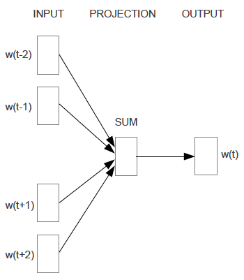
the Continuous Bag-of-Words model (CBOW)
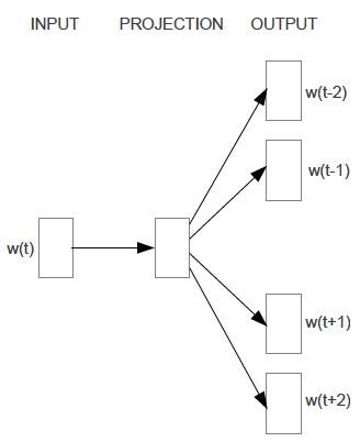
the Skip-Gram model (Section 3.1 and 3.2 in Mikolov et al.).

Algorithmically, these models are similar, except that

CBOW predicts target words (e.g. 'mat') from source context words ('the cat sits on the'),
the skip-gram does the inverse and predicts source context-words from the target words.

CBOW smoothes over a lot of the distributional information (by treating an entire context as one observation). For the most part, this turns out to be a useful thing for smaller datasets.
skip-gram treats each context-target pair as a new observation, and this tends to do better when we have larger datasets. We will focus on the skip-gram model in the rest of this tutorial.

Scaling up with Noise-Contrastive Training

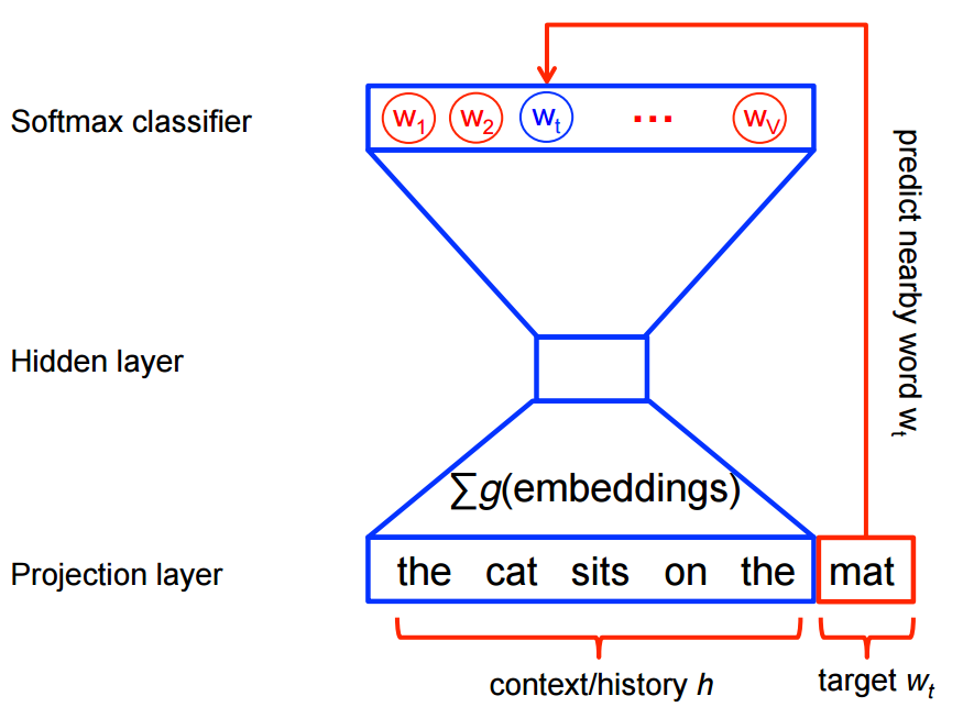
Neural probabilistic language models are traditionally trained using the maximum likelihood (ML) principle to maximize the probability of the next word wt (for "target") given the previous words h (for "history") in terms of a softmax function,

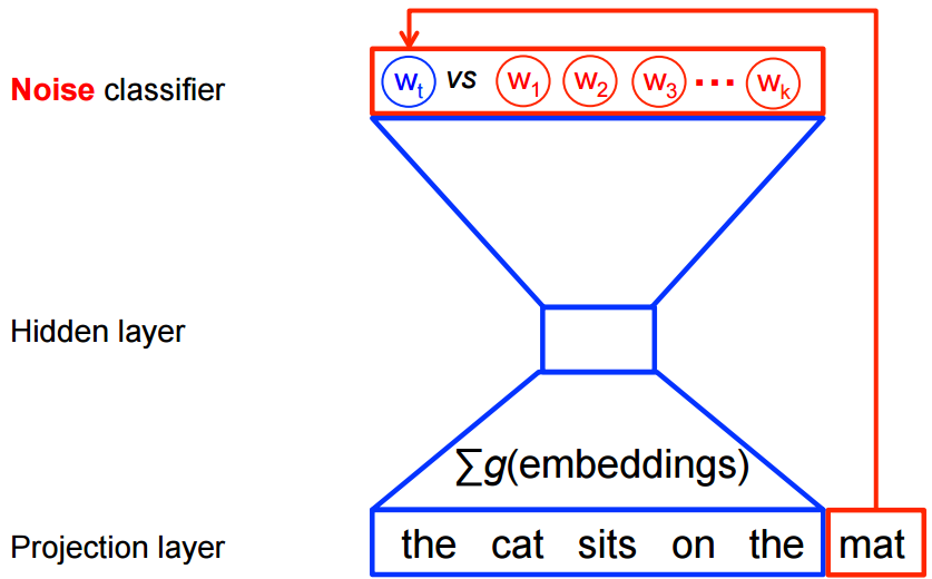
On the other hand, for feature learning in word2vec we do not need a full probabilistic model.

The CBOW and skip-gram models are instead trained using a binary classification objective (logistic regression) to discriminate the real target words w_t from k imaginary (noise) words w~,

in the same context. We illustrate this below for a CBOW model. For skip-gram the direction is simply inverted.

The Skip-gram Model

We can visualize the learned vectors by projecting them down to 2 dimensions using for instance something like the t-SNE dimensionality reduction technique.

When we inspect these visualizations it becomes apparent that the vectors capture some general, and in fact quite useful, semantic information about words and their relationships to one another.

It was very interesting when we first discovered that certain directions in the induced vector space specialize towards certain semantic relationships, e.g. male-female, verb tense and even country-capital relationships between words, as illustrated in the figure below (see also for example Mikolov et al., 2013).

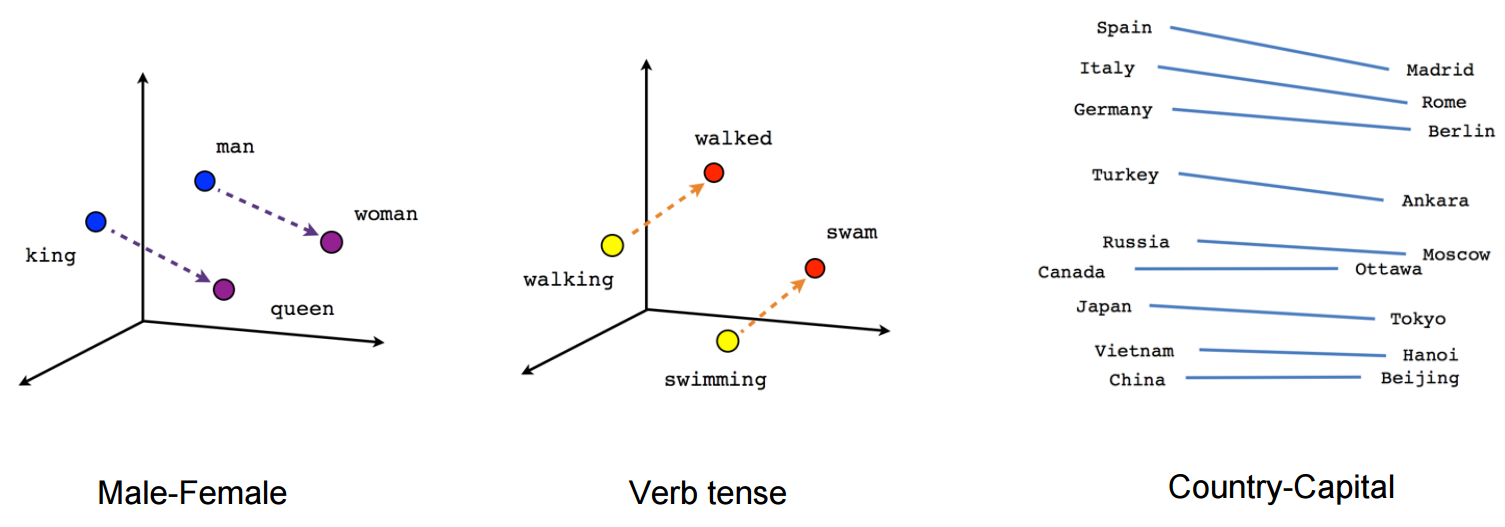
This explains why these vectors are also useful as features for many canonical NLP prediction tasks, such as part-of-speech tagging or named entity recognition (see for example the original work by Collobert et al., 2011 (pdf), or follow-up work by Turian et al., 2010).

But for now, let's just use them to draw pretty pictures!

Building the Graph

This is all about embeddings, so let's define our embedding matrix. This is just a big random matrix to start. We'll initialize the values to be uniform in the unit cube.

embeddings = tf.Variable(

    tf.random_uniform([vocabulary_size, embedding_size], -1.0, 1.0))

The noise-contrastive estimation loss is defined in terms of a logistic regression model. For this, we need to define the weights and biases for each word in the vocabulary (also called the output weights as opposed to the input embeddings). So let's define that.

nce_weights = tf.Variable(

  tf.truncated_normal([vocabulary_size, embedding_size],

                      stddev=1.0 / math.sqrt(embedding_size)))

nce_biases = tf.Variable(tf.zeros([vocabulary_size]))

Now that we have the parameters in place, we can define our skip-gram model graph. For simplicity, let's suppose we've already integerized our text corpus with a vocabulary

so that each word is represented as an integer (seetensorflow/examples/tutorials/word2vec/word2vec_basic.py for the details).

The skip-gram model takes two inputs. One is a batch full of integers representing the source context words, the other is for the target words. Let's create placeholder nodes for these inputs, so that we can feed in data later.

# Placeholders for inputs

train_inputs = tf.placeholder(tf.int32, shape=[batch_size])

train_labels = tf.placeholder(tf.int32, shape=[batch_size, 1])

Now what we need to do is look up the vector for each of the source words in the batch. TensorFlow has handy helpers that make this easy.

embed = tf.nn.embedding_lookup(embeddings, train_inputs)

Ok, now that we have the embeddings for each word,

we'd like to try to predict the target word using the noise-contrastive training objective.

# Compute the NCE loss, using a sample of the negative labels each time.

loss = tf.reduce_mean(

  tf.nn.nce_loss(weights=nce_weights,

                 biases=nce_biases,

                 labels=train_labels,

                 inputs=embed,

                 num_sampled=num_sampled,

                 num_classes=vocabulary_size))

Now that we have a loss node, we need to add the nodes required to compute gradients and update the parameters, etc. For this we will use stochastic gradient descent, and TensorFlow has handy helpers to make this easy as well.

# We use the SGD optimizer.

optimizer = tf.train.GradientDescentOptimizer(learning_rate=1.0).minimize(loss)

Training the Model

Training the model is then as simple as using a feed_dict to push data into the placeholders and calling tf.Session.run with this new data in a loop.

for inputs, labels in generate_batch(...):

  feed_dict = {train_inputs: inputs, train_labels: labels}

  _, cur_loss = session.run([optimizer, loss], feed_dict=feed_dict)

See the full example code in tensorflow/examples/tutorials/word2vec/word2vec_basic.py.

Visualizing the Learned Embeddings

After training has finished we can visualize the learned embeddings using t-SNE.

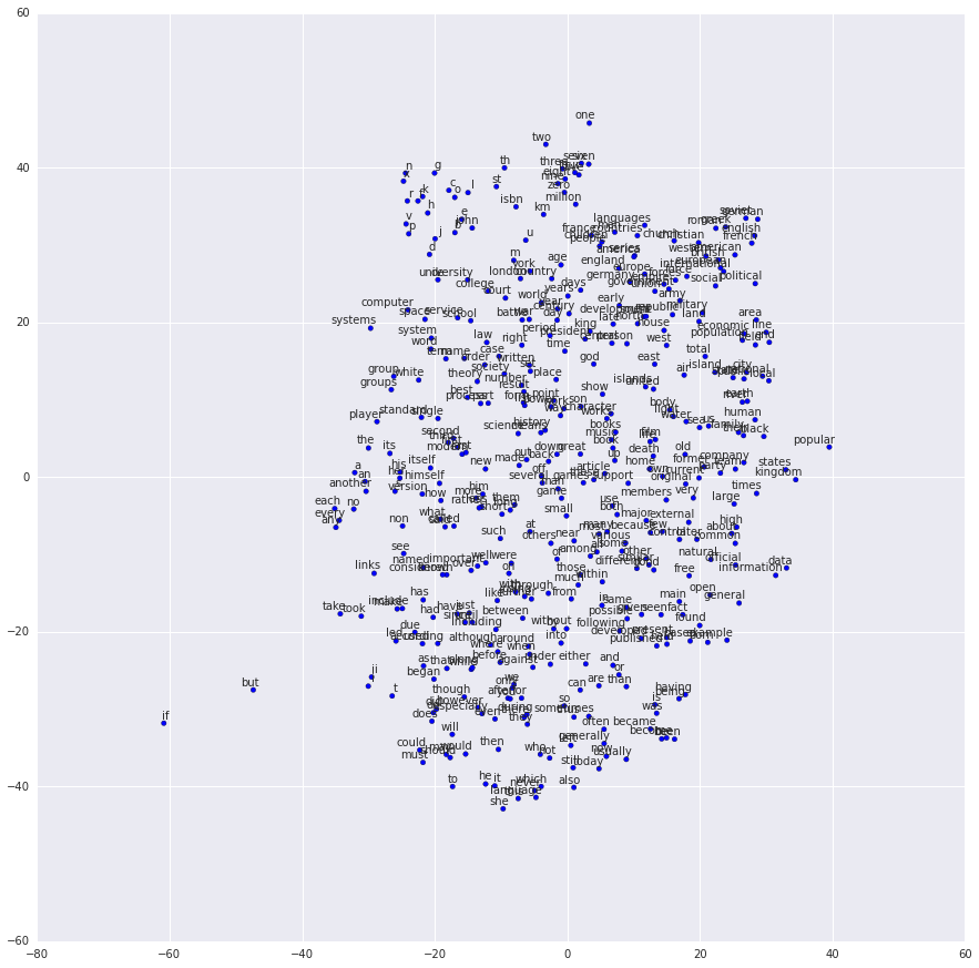
As expected, words that are similar end up clustering nearby each other.

For a more heavy weight implementation of word2vec that showcases more of the advanced features of TensorFlow, see the implementation in models/tutorials/embedding/word2vec.py.

Evaluating Embeddings: Analogical Reasoning

Embeddings are useful for a wide variety of prediction tasks in NLP. Short of training a full-blown part-of-speech model or named-entity model, one simple way to evaluate embeddings is to directly use them to predict syntactic and semantic relationships like king is to queen as father is to ?. This is called analogical reasoning and the task was introduced by Mikolov and colleagues. Download the dataset for this task from download.tensorflow.org.

To see how we do this evaluation, have a look at the build_eval_graph() and eval() functions inmodels/tutorials/embedding/word2vec.py.

The choice of hyperparameters can strongly influence the accuracy on this task. To achieve state-of-the-art performance on this task requires training over a very large dataset, carefully tuning the hyperparameters and making use of tricks like subsampling the data, which is out of the scope of this tutorial.

Optimizing the Implementation

Loss function change.

For example, changing the training objective is as simple as swapping out the call to tf.nn.nce_loss() for an off-the-shelf alternative such as tf.nn.sampled_softmax_loss().

If you have a new idea for a loss function, you can manually write an expression for the new objective in TensorFlow and let the optimizer compute its derivatives.

Run more efficiently

If you find your model is seriously bottlenecked on input data, you may want to implement a custom data reader for your problem, as described in New Data Formats. For the case of Skip-Gram modeling, we've actually already done this for you as an example in models/tutorials/embedding/word2vec.py.

Custom API for more performance

If your model is no longer I/O bound but you want still more performance, you can take things further by writing your own TensorFlow Ops, as described in Adding a New Op.

Again we've provided an example of this for the Skip-Gram case models/tutorials/embedding/word2vec_optimized.py. Feel free to benchmark these against each other to measure performance improvements at each stage.

Conclusion

In this tutorial we covered the word2vec model, a computationally efficient model for learning word embeddings. We motivated why embeddings are useful, discussed efficient training techniques and showed how to implement all of this in TensorFlow. Overall, we hope that this has show-cased how TensorFlow affords you the flexibility you need for early experimentation, and the control you later need for bespoke optimized implementation.