吴裕雄--天生自然 R语言开发学习：中级绘图（续二）

#------------------------------------------------------------------------------------#
# R in Action (2nd ed): Chapter 11                                                   #
# Intermediate graphs                                                                #
# requires packages car, scatterplot3d, gclus, hexbin, IDPmisc, Hmisc,               #
#                   corrgram, vcd, rlg to be installed                               #
# install.packages(c("car", "scatterplot3d", "gclus", "hexbin", "IDPmisc", "Hmisc",  #
#                    "corrgram", "vcd", "rld"))                                      #
#------------------------------------------------------------------------------------#

par(ask=TRUE)
opar <- par(no.readonly=TRUE) # record current settings

# Listing 11.1 - A scatter plot with best fit lines
attach(mtcars)
plot(wt, mpg,
     main="Basic Scatterplot of MPG vs. Weight",
     xlab="Car Weight (lbs/1000)",
     ylab="Miles Per Gallon ", pch=19)
abline(lm(mpg ~ wt), col="red", lwd=2, lty=1)
lines(lowess(wt, mpg), col="blue", lwd=2, lty=2)
detach(mtcars)

# Scatter plot with fit lines by group
library(car)
scatterplot(mpg ~ wt | cyl, data=mtcars, lwd=2,
            main="Scatter Plot of MPG vs. Weight by # Cylinders",
            xlab="Weight of Car (lbs/1000)",
            ylab="Miles Per Gallon", id.method="identify",
            legend.plot=TRUE, labels=row.names(mtcars),
            boxplots="xy")

# Scatter-plot matrices
pairs(~ mpg + disp + drat + wt, data=mtcars,
      main="Basic Scatterplot Matrix")

library(car)
library(car)
scatterplotMatrix(~ mpg + disp + drat + wt, data=mtcars,
                  spread=FALSE, smoother.args=list(lty=2),
                  main="Scatter Plot Matrix via car Package")

# high density scatterplots
set.seed(1234)
n <- 10000
c1 <- matrix(rnorm(n, mean=0, sd=.5), ncol=2)
c2 <- matrix(rnorm(n, mean=3, sd=2), ncol=2)
mydata <- rbind(c1, c2)
mydata <- as.data.frame(mydata)
names(mydata) <- c("x", "y")

with(mydata,
     plot(x, y, pch=19, main="Scatter Plot with 10000 Observations"))

with(mydata,
     smoothScatter(x, y, main="Scatter Plot colored by Smoothed Densities"))

library(hexbin)
with(mydata, {
  bin <- hexbin(x, y, xbins=50)
  plot(bin, main="Hexagonal Binning with 10,000 Observations")
})

# 3-D Scatterplots
library(scatterplot3d)
attach(mtcars)
scatterplot3d(wt, disp, mpg,
              main="Basic 3D Scatter Plot")

scatterplot3d(wt, disp, mpg,
              pch=16,
              highlight.3d=TRUE,
              type="h",
              main="3D Scatter Plot with Vertical Lines")

s3d <-scatterplot3d(wt, disp, mpg,
                    pch=16,
                    highlight.3d=TRUE,
                    type="h",
                    main="3D Scatter Plot with Vertical Lines and Regression Plane")
fit <- lm(mpg ~ wt+disp)
s3d$plane3d(fit)
detach(mtcars)

# spinning 3D plot
library(rgl)
attach(mtcars)
plot3d(wt, disp, mpg, col="red", size=5)

# alternative
library(car)
with(mtcars,
     scatter3d(wt, disp, mpg))

# bubble plots
attach(mtcars)
r <- sqrt(disp/pi)
symbols(wt, mpg, circle=r, inches=0.30,
        fg="white", bg="lightblue",
        main="Bubble Plot with point size proportional to displacement",
        ylab="Miles Per Gallon",
        xlab="Weight of Car (lbs/1000)")
text(wt, mpg, rownames(mtcars), cex=0.6)
detach(mtcars)

# Listing 11.2 - Creating side by side scatter and line plots
opar <- par(no.readonly=TRUE)
par(mfrow=c(1,2))
t1 <- subset(Orange, Tree==1)
plot(t1$age, t1$circumference,
     xlab="Age (days)",
     ylab="Circumference (mm)",
     main="Orange Tree 1 Growth")
plot(t1$age, t1$circumference,
     xlab="Age (days)",
     ylab="Circumference (mm)",
     main="Orange Tree 1 Growth",
     type="b")
par(opar)

# Listing 11.3 - Line chart displaying the growth of 5 Orange trees over time
Orange$Tree <- as.numeric(Orange$Tree)
ntrees <- max(Orange$Tree)
xrange <- range(Orange$age)
yrange <- range(Orange$circumference)
plot(xrange, yrange,
     type="n",
     xlab="Age (days)",
     ylab="Circumference (mm)"
)
colors <- rainbow(ntrees)
linetype <- c(1:ntrees)
plotchar <- seq(18, 18+ntrees, 1)
for (i in 1:ntrees) {
  tree <- subset(Orange, Tree==i)
  lines(tree$age, tree$circumference,
        type="b",
        lwd=2,
        lty=linetype[i],
        col=colors[i],
        pch=plotchar[i]
  )
}
title("Tree Growth", "example of line plot")
legend(xrange[1], yrange[2],
       1:ntrees,
       cex=0.8,
       col=colors,
       pch=plotchar,
       lty=linetype,
       title="Tree"
)                                          

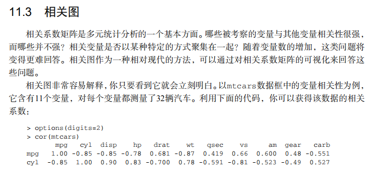
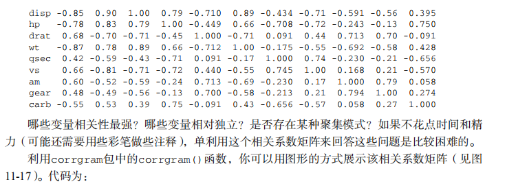
# Correlograms
options(digits=2)
cor(mtcars)

library(corrgram)
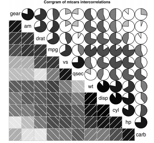
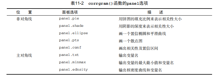
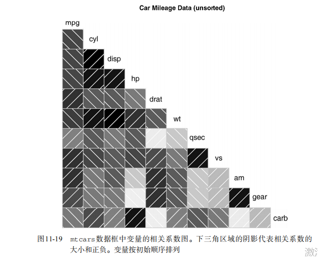
corrgram(mtcars, order=TRUE, lower.panel=panel.shade,
         upper.panel=panel.pie, text.panel=panel.txt,
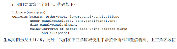
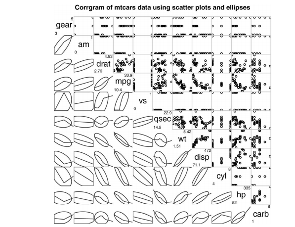
         main="Corrgram of mtcars intercorrelations")

corrgram(mtcars, order=TRUE, lower.panel=panel.ellipse,
         upper.panel=panel.pts, text.panel=panel.txt,
         diag.panel=panel.minmax,
         main="Corrgram of mtcars data using scatter plots
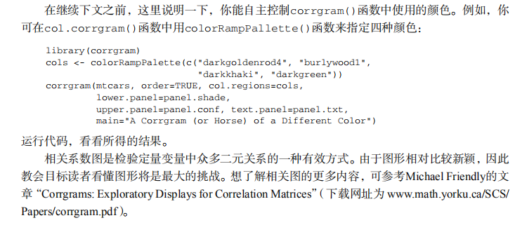
and ellipses")

cols <- colorRampPalette(c("darkgoldenrod4", "burlywood1",
                           "darkkhaki", "darkgreen"))
corrgram(mtcars, order=TRUE, col.regions=cols,
         lower.panel=panel.shade,
         upper.panel=panel.conf, text.panel=panel.txt,
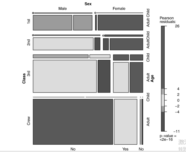
         main="A Corrgram (or Horse) of a Different Color")

# Mosaic Plots
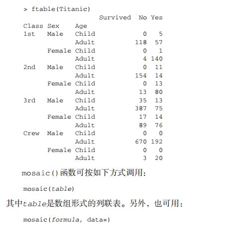
ftable(Titanic)
library(vcd)
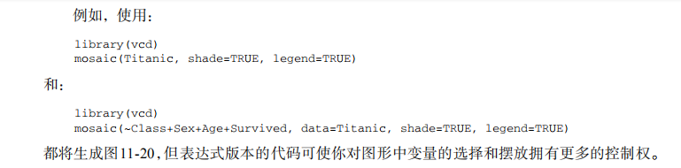
mosaic(Titanic, shade=TRUE, legend=TRUE)

library(vcd)
mosaic(~Class+Sex+Age+Survived, data=Titanic, shade=TRUE, legend=TRUE)

# type= options in the plot() and lines() functions
x <- c(1:5)
y <- c(1:5)
par(mfrow=c(2,4))
types <- c("p", "l", "o", "b", "c", "s", "S", "h")
for (i in types){
  plottitle <- paste("type=", i)
  plot(x,y,type=i, col="red", lwd=2, cex=1, main=plottitle)
}