Course Machine Learning Note
Machine Learning Note
Introduction
Introduction
What is Machine Learning?
Two definitions of Machine Learning are offered. Arthur Samuel described it as:"the filed of study that gives computers the ability to learn without being explicitly programmed." This is an older, informal definition.
Tom Mitchell provides a more modern definition:"A computer program is said to learn from esxperience E with respect to some class of tasks T and performance measure P, if its performance at tasks in T, as measured by P, improves with experience E."
Example: playing checkers
E=the experience of playing many games of checkers.
T=the task of playing checkers.
P=the probability that the program will win the next game.
In general, any machine learning problem can be assigned to ont of two broad classifications:
Supervised learning and Unsupervised learning
Supervised Learning
in supervised learning, we are given a data set and already know what our correct output should look like, having the idea that there is a relationship between the input and output.
Supervised learning problems are categorized into "regression" and "classification" problems. In a regression problem, we are trying to predict results within a continuous function, meaning that we are trying to map input variables to some continuous function. In a classification problem, we are instead trying to predict results in discrete output. In other words, we are trying to map input variables into discrete categories.
Example 1:
Give data about the size of houses on the real estate market, try to predict their price. Price as a function of size is a continuous output, so this is a regression problem.
We could turn this example into a classification problem by instead making our output about whether the house "sells for more or less than the asking price." Here we are classifying houses based on price into two discrete categories.
Example 2:
- Regression-Given a picture of a person, we have to predict their age on the basis of the given picture
- Classification-Given a patient with a tumor, we have to predict whether the tumor is malignant or benign.
Unsupervised Learning
Unsupervised learning allows us to approaach problems with little or no idea what our results should look like. We can derive structure from data where we don't necessarily know the effect of the variables.
We can derive this structure by clustering data based on relationships among the variables in the data.
With unsupervised learning there is no feedback based on the prediction results.
Example:
Clustering: Take a collectio of 1,000,000 different genes, and find a way to automatically group these genes into groups that are somehow similar or related by different variables, such as lifespan, location, roles, and so on.
Non-clustering: The "Cocktail Party Algorithm", allows you to find structure in a chaotic environment.(i.e identifying individual voices and music from a mesh of sounds at a cocktail party).
Linear Regression with One Variable
Model and Cost Function
Model Representation
To establish notation for future use, we'll use to denote the "input" variables(living area in this example), also called input features, and to denote the "output" or target variable that we are trying to predict(price). A pair(,) is called a training example, and the dataset that we'll be using to learn----- a list of m training examples(,);i=1,….,m is called a training set. Note that the usperscript (i) in the notation is simply an index into the training set, and has nothing to do with exponentitaion. We will also use X to denote the space of input values, and Y to denote the space of output values. In this example, X=Y=ℝ
To describe the the supervised learning problem slightly more formally, our goal is, given a training set, to learn a function h: X -> Y so that h(x) is a "good" predictor for the corresponding value of y. For historical reasons, this function h is called a hypothesis. Seen pictorially, the process is therefore like this:
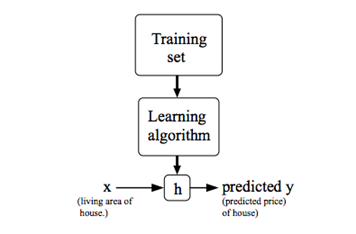
When the target variable that we're trying to predict is continuous, such as in our housing example, We call the learning problem a regression problem. When y can take on only a small number of discrete values(such as if,given the living area, we wanted to predict if a dwelling is a house or a apartment, say), we call it a classification problem.
Cost Function
We can measure the accuracy of our hypothesis function by using a cost function. This takes an average difference(actually a fancier version of an average) of all the results of the hypothesis with input from x's and the actual output y's

To break it apart, it is
Cost Function-Intuition I
if we try to think of it in visual terms, our training data set is scattered on the x-yplane. We are trying to make a straight line(defined by ) which passes through these scattered data points.
Our objective is to get the best possible line. The best possible line will be such so that the average squared vertical distances of the scattered points from the line will be the least. Ideally, the line should pass through all the points of our training data set. In such a case, the value of will be 0. The following example shows the ideal situation where we have a cost function of 0.
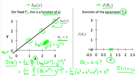
where ,we get a slope of 1 which goes through every single data point in our model. Conversely, where =0.5, we see the vertical distance from our fit to the data points increase.
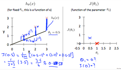
This increases our cost function to 0.58. Plotting serveral other points yields to the following graph:
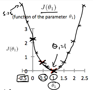
Thus as a goal, we should try to minimize the cost function. In this case =1 is our global minimum.
Cost Function-Intition II
A contour plot is a graph that contains many contour lines. A contour line of a two variable function has a constan value at all points of the same line. An example of such a graph is the one to the right below.
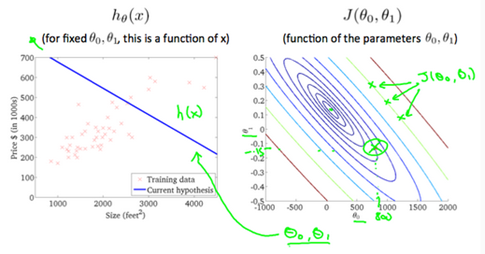
Taking any color and going along the 'circle', one would expect to get the same value of the cost function. For example, the three green points found on the green line above have the same value for and as a result, they are found along the same line. The circled x displays the value of the cost function for the graph on the leftt when . Taking another h(x) and plotting its contour plot, one gets the following graphs:
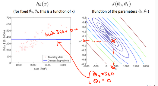
Whe , the value of in the contour plot gets closer to the center thus reducing the cost function error. Now giving our hypothesis function a slightly positive slope results in a better fit of the data.
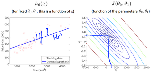
The graph above minimizes the cost function as much as possible and consequently the result of tend to be aroud 0.12 and 250 respectively. Plotting those values on our graph to the right seems to put our point in the center of the inner most 'circle'.
Parameter Learning
Gradient Descent
So we have our hypothesis function and we have a way of measuring how well it fits into the data. Now we need to estimate the parameters in the hypothesis function. That's where gradient descent comes in.
Imagine that we graph our hypothesis function based on its fields (actually we are graphing the cost function as a function of the parameter estimates). We are not graphing x and y itself, but the parameter range of our hypothesis function and the cost resulting from selecting a particular set of parameters.
We put on the x axis and on the y axis, with the cost function on the vertical z axis. The points on our graph will be the result of the cost function using our hypothesis with those specific theta parameters. The graph below depicts such a setup.
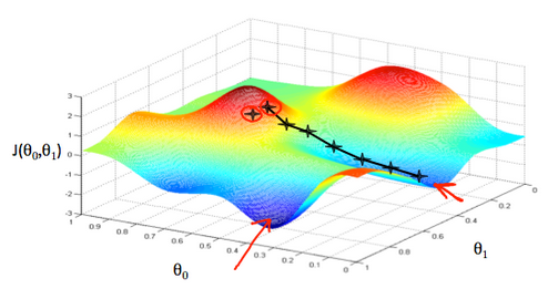
We will know that we have succeeded when our cost function is at the very bottom of the pits in our graph, I.e. when its value is the minimum. The red arrows show the minimum points in the graph.
The way we do this is by taking the derivative(the tangential line to a function) of our cost function. The slope(斜率) of the tangent(正切) is the derivative at that point and it will give us a direction to move towards. We make steps down the cost function in the direction with the steepest descent. The size of each step is determined by the parameter α, which is called the learning rate.
For example, the distance between each 'star' in the graph above represents a step determined by our parameter a. A smaller α would result in a smaller step and a large α results in a larger step. The direction in which the step is taken is determined by the partial derivative of . Depending on where one starts on the graph,one could end up at different poins. The image above shows us two different starting pints that end up in two different places.
The gradient descent algorithm is:
repeat until convergence:

where
j=0,1 represents the feature index number.
At each iteration j,one should simultaneously(同时) update the parameters  . Updating a specific parameter prior to calculating another one on the iteration would yield to a wrong implementation.

Gradient Descent Intuition
In this video we explored the scenario(方案) where we used one parameter and plotted its cost function to implement a gradient descent. Our formula for a single parameter was:
Repeat until convergence:

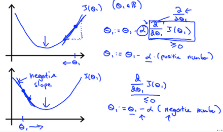
Regardless of slope's sign(符号) for ,eventually converges to its minimum value. The following graph show that when the slope is negative, the value of increases and when it is positive , the value of decreases.
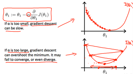
On a side note, we should adjust our parameter α to ensure that the gradient descent algorithm converges in a resonable time. Failure to converge or too much time to obtain the miimum value imply that our step size is wrong.
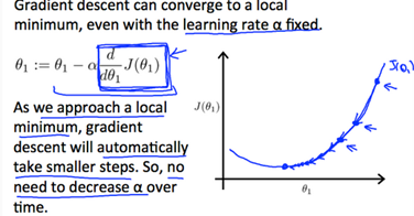
How does gradient descent converge with a fixed step size α?
The intuition(直觉) behind the convergence is that approaches 0 as we approach the bottom of our convex function. At the minimum , the derivative will always be 0 and thus we get:

Gradient Descent For Linear Regression
When specifically applied to the case of linear regression,a new form of the gradient descent equation(方程式) can be derived(衍生). We can substitute(替代) our actual cost function and our actual hypothesis function and modify the equation to:
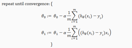
where m is the size of the training set, a constant that will be changing simultaneously with and are values of the given training set(data).
Note that we have separated out the two cases for into separate equations for ; and that for we are multiplying at the end due to the derivative. The following is a derivation of for a single example:
The point of all this is that if we start with a guess for our hypothesis and then repeatedly apply these gradient descent equations, our hypothesi will become more and more accurate.
So, this is simply gradient descent on the original cost function J. This mthod looks at every example in the entire training set on every step, and is called batch gradient descent. Note that, while gradient descent can be susceptible to local minima in general, the optimization problem we have posed here for linear regression has only one global, and no other local, optima(最适宜的); thus gradient descent always converges(assumig the learning rate a is not too large) to the global minimum. Indeed, J is a convex quadratic(二次) function.
The ellipses(椭圆) shown above are the contours of a quadratic function. Also shown is the trajectory(轨道) taken by gradient descent, which was initialized at (48,30). The x's in the figure (joined by straight lines) mark the successive values of θ that gradient descent went through as it converged to its minimum.
Linear Regression with Multiple Variables
Multivariate Linear Regression
Multiple Features
Linear regression with multiple variables is also known as "multivariate linear regression".
We now introduce notation(标记法) for equations where we can hava any number of input variables.

The multivariable form of the hypothesis function(假设函数) accommodating these multiple features is as follows:

In order to develop intuition(直觉) about this function, we can think about as the basic price of a house, as the price per square meter, as the price per floor, etc. will be the number of square meters in the house, the number of floors, etc.
Using the definition of matrix multiplication, our multivariable hypothesis function can be concisely represented as:

This is a vectorization(向量化) of our hypothesis function for one training example; see the lessons on vectorization to learn more.
Remark: Note that for convenience reasons in this course we assume =1 for ( ). This allows us to do matrix operations with theta and X. Hence making the two vectors 'ө' and match each other element-wise(that is,have the same number of elements:n+1).
Gradient Descent for Multiple Variables
The gradient descent equation itself is generally the same form; we just have to repeat it for our 'n' features:
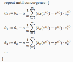
In other words:

The following image compares gradient descent with one variable to gradient descent with multiple variables:
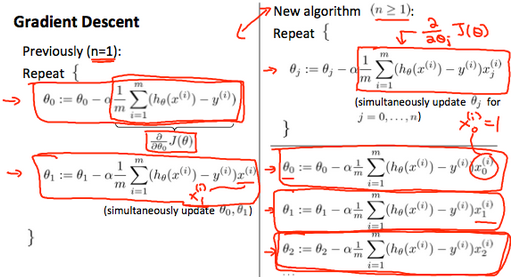
Gradient Descent in Practice I: Feature Scaling(特征缩放)
We canspeed up gradient descent by having each of our input values in roughly the same range. This is because ө will descend quickly on small ranges and slowly on large ranges, and so will oscillate(震荡) inefficiently down to the optimum when the variables are very uneven.
The way to prevent this is to modify the ranges of our input variables so that they are all roughly(大体上) the same. Ideally:
or
These aren't exact requirements; we are only trying to speed things up. The goal is to get all input variables into roughly one of these ranges, give or take a few.
Two techniques to help with this are feature scaling(特征缩放) and mean normalization(均值归一化处理). Feature scaling involves(牵涉) dividing the input values by the range(i.e the maximum value minus the minmum value) of the input variable, resulting in a new range of just 1. Mean normalization involves subtracting the average value for an input variable from the values for that input variable resulting in a new average value for the input variable of just zero. To implement both of these techniques, adjust your input values as shown in this formula:

where is the average of all the values for feature(i) and is the range of values(max-min), or is the standard deviation(绝对偏差).
Note that dividing by the range, or dividing by the standard deviation, give different results. The quizzes in this course use range, the programming exercises use standard deviation.
For example, if represents housing prices with a range of 100 to 200 and a mean value of 1000, then

Gradient Descent in Practice II: Learning Rate
Debugging gradient descent. Make a plot with number of iterations on the x-axis. Now pot the cost function, J(ө) over the number of iterations of iterations of gradient descent. if J(ө) ever increase, then you probably need to decrease α.
Automatic convergence test. Declare convergence if J(ө) decreases by less then E in one iteration, where E is some small value such as . However in practice it's difficult to choose this threshold(阈值) value.
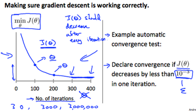
It has been proven that if learning rate α is sufficiently small, then J(ө) will decrease on every iteration.
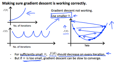
To summarize:
if α is too small: slow convergence.
if α is too large: may not decrease on every iteration and thus may not converge.
Features and Polynomial(多项式) Regression
We can improve our features and the form of our hypothesis function in a couple different ways.
We can combine multiple features into one. For example, we can combine into a new feature by taking *.
Polynomial Regression
Our hypothesis function need not be linear(a straight line) if that does not fit the data well.
We can change the behavior or curve of our hypothesis function by making it a quadratic, cubic or square root function (or any other form).
For example, if our hypothesis function is

then we can create additional features base on , to get the quadratic function

or the cubic function

In the cubic version, we have created new features and where = and =.
To make it a square root function, we could do:

One important thing to keep in mind is, if you choose your features this way then feature scaling becomes very important.
eg. if has range 1-1000 then range of becomes 1-1000000 and that of becomes 1-10000000
Computing parameters Analytically
Normal Equation(正规方程)
Gradient descent gives one way of minimizing J. Let's discuss a second way of doing so, this time performing the minimization explicitly and without resorting to an iterative algorithm. In the "Normal Equation" method, we will minimize J by explicitly taking tis derivatives with respect to θj's, and setting them to zero. This allows us to find the optimum theta without iteration. The normal equation formula is given below:

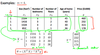
There is no need to do feature scaling with the normal equation.
The following is a comparison of gradient descent and the normal equation:
|
Gradient Descent |
Normal Equation |
|
Need to choose alpha |
No need to choose alpha |
|
Needs many iterations |
No need to iterate |
|
O(kn^2) |
O(n^3),need to calculate inverse of |
|
Works well when n is large |
Slow if n is very large |
with the normal equation, computing the inversion has complexity O(n^3). So if we have a very large number of features, the normal equation will be slow. In practice, when n exceeds 10,000 it might be a good time to go from a normal solution to an iterative process.
Normal Equation Noninvertibility(正规方程不可逆性)
When implementing the normal equation in octave we want to use the 'pinv' function rather then 'inv'. The 'pinv' function will give you a value of ө even if is not inertible.
if is noninvertible, the common causes might be having:
- Redundant(多余) features, where two features are very closely related(i.e. they are linearly dependent)
- Too many features(e.g. m<=n). In this case delete some features or use "regularization"
Solution to the above problems include deleting a feature that is linearly dependent with another or deleting one or more features when there are too many features.
Logistic Regression
Classification and Representation
Classification
To attempt classification, one method is to use linear regression and map all predictions greater than 0.5 as 1 and all less than 0.5 as 0. However, this method doesn't work well because classification is not actually a linear.
The classification problem is just like the regression problem, except that the values y we now want to predict take on only a small number of discrete values. For now, we will focus on the binary classification problem in which y can take on only two values, 0 and 1. (Most of what we say here will also generalize to the multiple-class case.) For instance, if we are trying to build a spam classifier for email, then may be some features of a piece of email, and y may be 1 if it is a piece of spam mail, and 0 otherwise. Hence, . 0 is also called the negative class, and 1 the positive class, and they are sometimes also denoted by the symbols "-" and "+". Give , the corresponding is also called the label for the training example.
Hypothesis Representation(假说表示)
We could approach the classification problem ignoring the fact that y is discrete-valued, and use our old linear regression algorithm to try to predict y given x. However, it is easy to construct examples where this method performs very poorly. Intuitively(直觉的), it also dosen't make sense for to take values larger than 1 or smaller than 0 when we know that . To fix this, let's change the form for our hypotheses to satisfy . This is accomplished by plugging x into the Logistic Function.
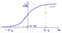
Our new form uses the "Sigmoid Function", also called the "Logistic Function":

z=
The following image shows us what the sigmoid function looks like:

The function g(z), shown here, maps any real number to the (0,1) interval(间隔), making it useful for transforming an arbitrary(随意)-value function into a function better suited for classification.
will give us the probability that our output is 1. For example, =0.7 gives us a probability of 70% that our output is 1. Our probability that our prediction is just the complement of our probability that it is 1 (e.g. if probability that it is 1 is 70%, then the probability that it is 0 is 30%).

Decision Boundary(判定边界)
In order to get our discrete 0 or 1 classification, we can translate the output of the hypothesis function as follows:

The way our logistic function g behaves is that when its input is greater than or equal to zero, its output is greater than or equal to 0.5:

Remember.

So if our input to g is x, then that means:

From these statements we can now say:

The decision bounday is the line that separates the area where y=0 and where y=1. It is created by our hypothesis function.
Example:
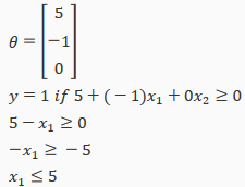
In this case, our decision boundary is a straight vertical line placed on the graph where x1=5, and everything to the left of that denoteds y=1, while everything to the right denotes y=0.
Again, the input to the sigmoid function g(z) (e.g. x) doesn't need to be linear, and could be a function that describes a circle(e.g.  ) or any shape to fit our data.
Logistic Regression Model
Cost Function
We cannot use the same cost function that we use for linear regression because the Logistic Function will cause the output to be wavy, causing many local optima. In other words, it will not be a convex function.
Instead, our cost function for logistic regression looks like:
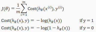
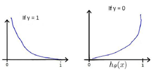

If our correct answer 'y' is 0, then cost function will be 0 if our hypothesis function also outputs 0. If our hypothesis approaches 1, then the cost function will approach infinity.
If our correct answer 'y' is 1, then the cost function will be 0 if our hypothesis function outputs 1. If our hypothesis approaches 0, then the cost function will approach infinity.
Note that writing the cost function in this way guarantees that J(θ) is convex for logistic regression.
Simplified Cost Function and Gradient Descent
We can compress our cost function's two conditional cases into one case:

Notice that when y is equal to 1, then the second term (1-y)log(1-(x)) will be zero and will not affect the result. If y is equal to 0, then the first term –ylog() will be zero and will not affect the result.
We can fully write out our entire cost function as follows:

A vectorized implementation is:

Gradient Descent
Remember that the general form of gradient descent is:

We can work out the derivative part using calculus to get:

step-by-step

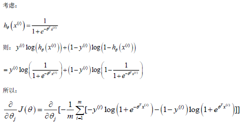
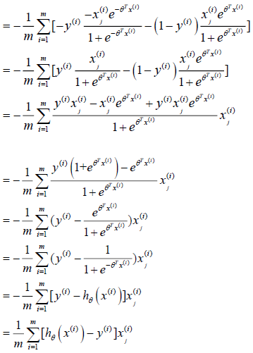
Notice that this algorithm is identical to the one we used in linear regression.
We still have to simultaneously update all value in theta.
A vectorized implementation is:

Advanced Optimization
"Conjugate gradient","BFGS",and "L-BFGS" are more sophisticated, faster ways to optimize ө that can be used instead of gradient descent. We suggest that you should not write these more sophisticated algorithms yourself(unless you are an expert in numerical computing) but use the libraries instead, as they're already tested and highly optimized. Octave provides them.
We first need to provide a function that evaluates the following two functions for a given input value ө:

We can write a single function that returns both of these:

Then we can use octave's "fminunc()" optimization algorithm along with the "optimset()" function that creates an object containing the options we want to send to "fminunc()".

We give to the function "fminunc()" our cost function, our initial vector of theta values, and the "options" object that we created beforehand.
Multicalss Classification
Multiclass Classification: One-VS-all
Now we will approach the classification of data whenwe have more than two categories. Instead of y={0,1} we will expand our definition(定义) so that y={0,1…n}.
Since y={0,1…n}, we divide our problem into n+1 (+1 because the index stars at 0) binary classification problems; in each one, we predict the probability that 'y' is a member of one our classes.
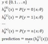
We are basically choosing one class and then lumping(把…归并在一起) all the others into a single second class. We do this repeatedly, applying binary logistic regression to each case, and then use the hypothesis that returned the highest value as our prediction.
The following image shows how one could classify 3 classes:

Solving the Problem of Overfitting
The problem of Overfitting(过拟合)
Consider the problem of predicting y from . The leftmost figure below shows the result of fitting a to a dataset. We see that the data doesn't really lie on straight line, and so the fit is not very good.

Instead, if we had added an extra feature , and fit , then we obtain a slightly better fit to the data(See middle figure). Naively, it might seem that the more feature we add, the better. However, there is also a danger in adding too many features: The rightmost figure is the result of fitting a order polynomial . We see that even though the fitted curve passes through the data perfectly, we would not expect this to be a very good predictor of, say, housing prices(y) for different living areas(x). Without formally defining what these terms mean, we'll say the figure on the left shows an instance of underfitting---in which the data clearly shows structure not captured by the model ----- and the figure on the right is an example of overfitting.
Underfitting, or high bias, is when the form of our hypothesis function h maps poorly to the tread of data. It is usually caused by a function that is too simple or uses too few features. At the other extreme, overfitting, or high variance, is caused by a hypothesis function that fits the available data but does not generalize well to predict new data. It is usually caused by a complicated function that creates a lot of unnecessary curves and angles unrelated to the data.
This terminology(术语) is applied to both linear and logistic regression. There are two main options to address the issue of overfitting:
- Reduce the number of features:
Manually select which features to keep.
Use a model selection algorithm
- Regularization(正则化)
keep all the feature, but reduce the magnitude(大量的) of parameters
Regularization works well when we have a lot of slightly useful features.
Cost Function
If we have overfitting from our hypothesis function, we can reduce the weight that some of the terms in our function carry by increasing their cost.
Say we wanted to make the following function more quadratic(二次的):

We'll want to eliminate the influence of and . without actually getting rid of these features or changing the form of our hypothesis, we can instead modify our cost function:

We've added two extra terms at the end to inflate the cost of and . Now, in order for the cost function to get close to zero, we will have to reduce the values of and to near zero. This will in turn greatly reduce the values of and in our hypothesis function. As a result, we see that the new hypothesis(depicted by the pink curve) looks like a quadratic function but fits the data better due to the extra small terms and
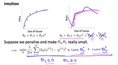
We could also regularize all of our theda parameters in a single summation as:

The λ, or lambda, si the regularization parameter. It determines how much the costs of our theta parameters are inflated(膨胀).
Using the above cost function with the extra summation, we can smooth the output of our hypothesis function to reduce overfitting. If lambda is chosen to be too laarge, it may smooth out the function too much and cause underfitting. Hence, what would happen if λ=0 or is too small?
Regularized Linear Regression
We can apply regularization to both linear regression and logistic regression. We will approach linear regression first.
Gradient Descent
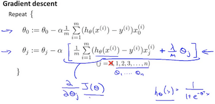
We will modify our gradient descent function to separate out from the rest of the parameters because we do not want to penalize(对…予以惩罚) .

The term performs our regularization. With some manipulation our update rule can also be represented as:

The first term in the above equation, will always be less than 1. Intuitively you can see it as reducing the value of by some amount on every update. Notice that the second term is now exactly the same as it was before.
Normal Equation(正规方程)
Now let'a approach regularization using the alternate method of the non-iterative normal equation.
To add in regularization, the equation is the same as our original, except that we add another term inside the parentheses:
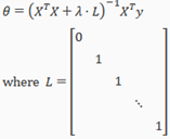
L is a matrix with 0 at the top left and 1's down the diagonal, with 0's everywhere else. It should have dimension (n+1)*(n+1). Intuitively, this is the identity matrix(though we are not including x0),multiplied with a single real number λ.
Recall that if m<n, then is non-invertible. However, when we add the term λ⋅L, then becomes invertible.
Regularized Logistic Regression
We can regularize logistic regression in a similar way that we regularize linear regression. As a result, we can avoid overfitting. The following image shows how the regularized function, dispalyed by the pink line, is less likely to overfit then the non-regularied function represented by the blue line:
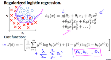
Cost Function
Recall that our cost function for logistic regression was:

We can regularize this equation by adding a term to the end:

The second sum, means to explicitly exclude the bias term, I.e the vector is indexed from 0 to n(holding n+1 values, through ), and this sum explicitly skips , by running from 1 to n, skipping 0. Thus, when computing the equation, we should continuously update the two following equations:
Neural Networks:Representation
Neural Networks
Model Representation I
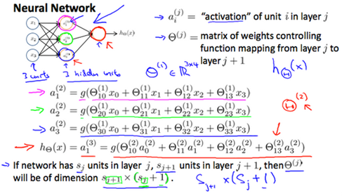
Let's examine how we will represent a hypothesis function using neural networks. At a very simple level, neurons are basically computational units that take inputs(dendrites树突)as electrical inputs(called "spikes") that are channeled to outputs(axons). In our model, our dendrites are like the input features , and the output is the result of out hypothesis function. In this model our input node is sometimes called the "bias unit". It is always equal to 1. In neural networks, we use the same logistic function as in classification, , yet we sometimes call it a sigmoid(logistic) activation function(激励函数). In this situation, our "theta" parameters are sometimes called "weights".
Visually, a simplistic representation looks like:

Our input nodes(layer 1), also known as the "input layer", go into another node(layer 2), which finally outputs the hypothesis function, known as the "output layer".
We can have intermediate layers of nodes between the input and output layers called the "hidden layers".
In this example, we label these intermediate or "hidden" layer nodes and call them "activation units"

If we had one hidden layer, it would look like:

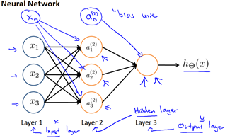
The values for each of the "activation" nodes is obtained as follows:

This is saying that we compute our activation nodes by using a 3*4 matrix of parameters. We apply each row of the parameters to our inputs to obtain the value for one activation node. Our hypothesis output is the logistic function applied to the sum of the values of our activation nodes, which have been multiplied by yet another parameter matrix containing the weights for our second layerof nodes.
Each layer gets its own matrix of weights,
The dimensions of these matrices of weights is determined as follows:
If network has units in layer j and units in layer j+1, then will be of dimension *(+1).
The +1 comes from the addition in of the "bias nodes", and . In other words the output nodes will not include the bias nodes while the inputs will. The following image summarizes our model representation.
Model Representation II
To re-iterate, the following is an example of a neural network:

In this section we'll do a vectorized implementation of the above functions. We're going to define a new variable that encompasses the parameters inside our g function. In our previous example if we replaced by the variable z for all the parameters we would get:

In other words, for layer j=2 and node k, the variable z will be:

The vector representation of x and is:

Setting x=, we can rewrite the equation as:

We are multiplying our matrix with dimensions *(n+1)(where is the number of our activation nodes) by our vactor with height (n+1). This gives us our vector with height . Now we can get a vector of our activation nodes for layer j as follows:

Where our function can be applied element-wise to our vector
We can then add a bias unit (equal to 1) to layer j after we have computed . This will be element and will be equal to 1. To compute our final hypothesis, let's first conpute another z vector:

We get this final z vector by multiplying the next theta matrix after with the values of all the activation nodes we just got. This last theta matrix will have only one row which is multiplied by one column so that our result is a single number. We then get our final result with:

Notice that in this last step, between layer j and layer j+1, we are doing exactly the same thing as we did in logistic regression. Adding all these intermediate layers in neural networks allows us to more elegantly produce interesting and more complex non-linear hypotheses.
Application
Examples and Intuitions I
A simple example of applying neural networks is by predicting , which is the logical 'and' operator and is only true if both are 1.
The graph of our functions will look like:

Remember that is our bias variable and is always 1.
Let's set our first matrix as:

This will cause the output of our hypothesis to only be positive if both are 1. In other words:
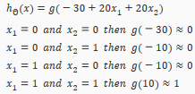
So we have constructed one of the fundamental operations in computers by using a small neural network rather than using an actual AND gate. Neural networks can also be used to simulate all the other logical gates. The following is an example of the logical operator 'OR', meaning either is true or is true, or both:
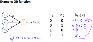
Where g(z) is the following:
Examples and Intuitions II
The matrices for AND, NOR, and OR are:
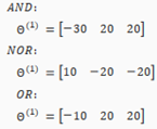
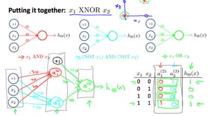
We can combine these to get the XNOR logical operator(which gives 1 if and are both 0 or both 1).

For the transition between the first and second layer, we'll use a matrix that combines the values for AND and NOR:

For the transition between the second and third layer, we'll use a matrix that uses the value for OR:

Let's write out the values for all our nodes:

And there we have the XNOR operator using a hidden layer with two nodes! The following summarizes the above algorithm:
Multiclass Classification
To classify data into multiple classes, we let our hypothesis function return a vector of values. Say we wanted to classify our data into one of four categories. We will use the following example to see how this classification is done. This algorithm takes as input an image and classifies it accordingly:

We can define our set of resulting classes as y:

Each represents a different image corresponding to either a car, pedestrian, truck, or motorcycle. The inner layers, each provide us with some new information which leads to our final hypothesis function. The setup looks like:

Our resulting hypothesis for one set of inputs may look like:

In which case our resulting class is the third one down, or 3, which represents the motorcycle.
Neural Networks: Learning
Cost Function and Backpropagation
Cost Function
Let's first define a few variables that we will need to use:
L=total number of layers in the network
=number of units(not counting bias unit) in layer l
K= number of output units/classes
Recall that in neural networks, we may have many output nodes. We denote k as being a hypothesis that results in the output. Our cost function for neural networks is going to be a generalization of the one we used for logistic regression. Recall that the cost function for regularized logistic regression was:

For neural networks, it is going to be slightly more complicated:
 We have added a few nested(嵌套) summations(总和) to account for our multiple output nodes. In the fist part of the equation, before the square brackets, we have an additional nested summation that loops through the number of output nodes.
In the regularization part, after the square brackets, we must account for multiple theta matrices. The number of columns in our current theta matrix is equal to the number of nodes in the next layer (excluding the bias unit). As before with logistic regression, we square every term.
Node:
The double sum simply adds up the loogistic regression costs calculated for each cell in the output layer
The triple sum simply adds up the squares of all the individual in the entire network.
The i in the triple sum does not refer to training example i.
Backpropagation Algorithm
"Backpropagation" is neural-network terminology for minimizing our cost function, just like what we were doing with gradient descent in logistic and linear regression. Our goal is to compute:

That is, we want to minimize our cost function J using an optimal set of parameters in theta. In this section we'll look at the equations we use to compute the partial derivative of :

To do so, we use the following algorithm:
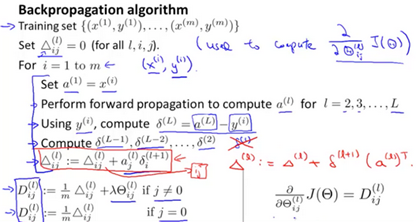
Back propagation Algorithm
Given training set {()…()}
- Set for all (l,I,j),(hence you end up having a matrix full of zeros)
For training example t=1 to m:
- Set
- Perform forward propagation to compute for l=2,3,…,L
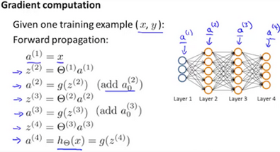
- Using , comupte
Where L is our total number of layers and is the vector of outputs of the activation units for the last layer. So our "error values" for the last layer are simply the difference of our actual results in the last layer and the correct outputs in y. To get the delta values of the layers before the last layer, we can use an equation that steps us back from right to left:
- Compute
The delta values of layer l are calculated by multiplying the delta values in the next layer with the delta matrix of layer l. We then element-wise multiply that with a function called , or g-prime, which is the derivative of the activation function g evaluated with the input values given by .
The g-prime derivative terms can also be written out as:
- or with vectorization,
Hence we update our new matrix.

The capital-delta matrix D is used as an "accumulator" to add up our values as we go along and eventually compute our partial derivative. Thus we get

Backpropagation Intuition
Recall that the cost function for a neural network is:

If we consider simple non-multiclass classification(k=1) and disregard regularization, the cost is computed with:

Intuitively, is the "error" for (unit j in layer l). More formally, the delta values are actually the derivative of the cost function:

Recall that our derivative is the slope of a line tangent to the cost function, so the steeper the slope the more incorrect we are. Let us consider the following neural network below and see how we could calculate some :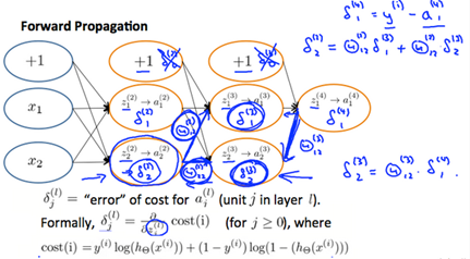
In the image above, to calculate , we multiply the weights and by their respective(各自的) vlues found to the right of each edge. So we get . To calculate every single possible , we could start from the right of diagram.
Backpropagation in Practice
Implementation Note: Unrolling Parameters
With neural networks, we are working withsets of matrices:

In order to use optimizing functions such as "fminunc()", we will want to "unroll" all the elements and put them into one long vector:
thetaVector = [ Theta1(:); Theta2(:); Theta3(:); ]
deltaVector = [ D1(:); D2(:); D3(:) ]
If the dimensions of Theta1 is 10*11, Theta2 is 10*11 and Theta3 is 1*11, then we can get back our original matrices from the "unrolled" versions as follows:

To summarize:
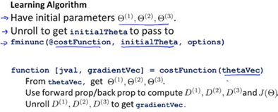
Gradient Checkong
Gradient checking will auusure that our backpropagation works as intended. We can approximate the derivative of our cost function with:

With multiple theta matrices, we can approximate the derivative with respect to as follows:

A small value for such as , guarantees that the math works out properly. If the value for is too small, we can end up with numerical problems.
Hence, we are only adding or subtracting epsilon to the matrix. In octave we can do it as follows:

We previously saw how to calculate the deltaVector. SO once we compute our gradApprox vector, we can check that gradApproxdeltaVector.
Once you have verified once that your backpropagation algorithm is correct, you don't need to compute gradApprox again. The code to compute gradApprox can be very slow.
Random Initialization
Initializing all theta weights to zero does not work with neural networks. When we backpropagation, all nodes will update to the same value repeatedly. Instead we can randomly initialize our weights for our matrices using the following method:
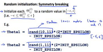
Hence, we initialize each to a random value between[-]. Using the above formula guarantees that we get the desired bound. The same procedure applies to all the . Below is some workong code you could use to experiment.

Rand(x,y) is just a function in octave that will initialize a matrix of random real numbers betweeen 0 and 1.
Putting it Together
First pick a network architectore; choose the layout of your neural network, including how many hidden units in each layer and how many layers in total you want to have.
- Number of input units=dimension of features
- Implement forward propagation to get for any
- Implement the cost function
- Implement backpropagation to compute partial derivatives
- Use gradient checking to confirm that your backpropagation works. Then disable gradient checking.
- Using gradient descent or a built-in optimization function to minimize the cost function with the weights in theta.
When we perform forward and back propagation, we loop on every training example:

The following image gives us an intuition of what is happening as we are implementing our neural network:
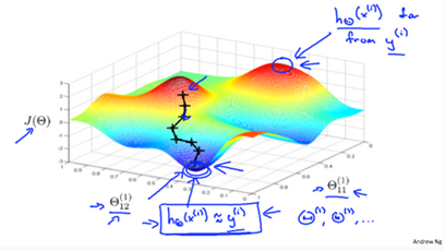
Ideally, you want . This will minimize our cost function. However, keep in mind that is not convex and thus we end up in a local minimum instead.
derivation process
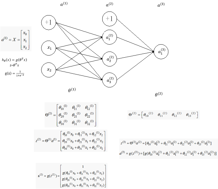
下面我们从一个简单的例子入手考虑如何从数学上计算代价函数的梯度,考虑如下简单的神经网络,该神经网络有三层神经元,对应的两个权重矩阵,为了计算梯度我们只需要计算两个偏导数即可:
首先计算第二个权重矩阵的偏导数,即
首先需要在之间建立联系,很容易可以看到的值取决于,而,而又是由取sigmoid得到,最后,所以他们之间的联系可以如下表示:

按照求导的链式法则,我们可以先求对的导数,然后乘以对的导数,即
由于
不难计算
令
上式可以重写为
接下来仅需要计算即可,由于
由
忽略前面的

得
这里只对一个example推导,最后累加即可
因此
,计算过程见附录,得
至此我们得到了
接下去我们需要求的偏导数,的依赖关系如下:

根据链式求导法则有
分别计算等式右边的三项可得
带入后得
令
上式可以重写为
将上面的结果放在一起,我们得到对两个权重矩阵的偏导数为:
观察上面的四个等式,我们发现
- 偏导数可以由当层神经元向量与下一层的误差向量相乘得到
- 当前层的误差向量可以由下一层的误差向量与权重矩阵的乘积得到
所以可以从后往前逐层计算误差向量,然后通过简单的乘法运算得到代价函数对每一层权重矩阵的偏导数。
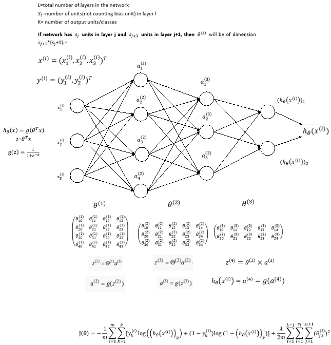
假设我们有m个训练example,L层神经网络,并且此处考虑正则项,即
初始化:设置(理解为对第l层的权重矩阵的偏导累加值)
For i=1:m
设置 a(1)=X
通过前向传播算法(FP)计算对各层的预测值,其中l=1,2,3,4…,L
计算最后一层的误差向量,利用后向传播算法(BP)从后至前逐层计算误差向量,计算公式为
更新
End//
计算梯度:


Advice for Applying Machine Learning
Evaluating a Learning Algorithm
Evaluating a Hypothesis
Once we have done some trouble shooting for errors in our predictions by:
- Getting more training examples
- Trying smaller sets of features
- Trying additional features
- Trying polynomial features
- Increasing or decreasing λ
We can move on to evaluate our new hypothesis.
A hypothesis may have a low error for the training examples but still be inaccurate(because of overfitting). Thus, to evaluate a hypothesis, given a dataset of training examples, we can split up the data into two sets: a training set and a test set. Typically, the training set consists of 70% of your data and the test set is the remaining 30%.
The new procedure using these two sets in then:
- Learn and minimize using the training set
- Compute the test set error
The test set error
For linear regression:

For classification~ Misclassification error (aka 0/1 misclassification error):
This gives us a binary 0 or 1 error result based on a misclassification. The average test error for the test set is:

This gives us the proportion of the test data that was misclassified.
Model Selection and Train/Validation/Test Sets
Just because a learning algorithm fits a training set well, that does not mean it is a good hypothesis. It could over fit and as a result your predictions on the test set would be poor.
The error of your hypothesis as measured on the data set with wich you trained the parameters will be lower than the error on any other data set.
Given many models with different polynomial degrees, we can use a systematic approach to identify the 'best' function. In order to choose the model of your hypothesis, you can test each degree of polynomial and look at the error result.
One way to break down our dataset into the three sets is:
- Traning set:60%
- Cross validation set:20%
- Test set:20%
We can now calculate three separate error values for the three different sets using the following method:
Optimize the parameters in using the training set for each polynomial degree.
Find the polynomial degree d with the least error using the cross validation set.
Estimate the generalization error using the test set with ,(d= theta from polynomial with lower error);
This way, the degree of the polynomial d has not been trained using the test set.
Bias vs. Variance
Diagnosing Bias vs. Variance
In this section we examine the relationship between the degree of the polynomial d and the underfitting or overfitting of our hypothesis.
- We need to distinguish whether bias or Variance is the problem contributing to bad predicitons.
- High bias is underfitting and high variance is overfitting. Ideally, we need to find a golden mean between these two.
The training error will tend to decrease as we increase the degree d of the polynomial.
At the same time, the cross validation error will tend to decrease as we increase d up to a point, and then it will increase as d is increased, forming a convex curve.
High bias (underfitting): both and will be high. Also,
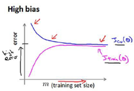
High variance(overfitting): will be low and will be much greater than .
The is summarized in the figure below:

Regularization and Bias/Variance

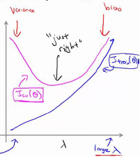
In the figure above, we see that as increase, our fit becomes more rigid. On the other hand, asapproaches 0, we tend to over overfit the data. So how do we choose our parameter to get it 'just right'? in order to choose the model and regularization term,We need to:
- Create a list of lambdas(i.e. );
- Create a set of models with different degrees or any other variants.
- Iterate through the and for each go through all the models to learn some .
- Compute the cross validation error using the learned (computed with) on the without regularization or.
- Select the best combo that produces the lowest error on the cross validation set.
- Using the best combo and, apply it on to see if it has a good generalization of the problem.
Learning Curves
Training an algorithm on a very few number of data points(such as 1,2 or 3) will easily have 0 errors because we can always find a quadratic curve that touches exactly those number of points. Hence:
- As the training set gets larger, the error for a quadratic function increase.
- The error value will plateau out after a certain m, or training set size.
Experiencing high bias:
Low training set size: causes and to be low and to be high.
Large training set size: causes both and to be high with .
If a learning algorithm is suffering from high bias, getting more training data will not(by itself) help much.
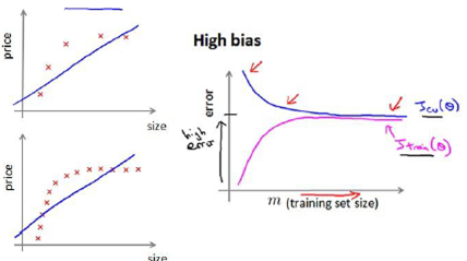
Experiencing high variance:
Low training set size: will be low and will be high.
Large training set size: increase with training set size and continues to decrease without leveling off. Also, but the difference betwewn them remains significant.
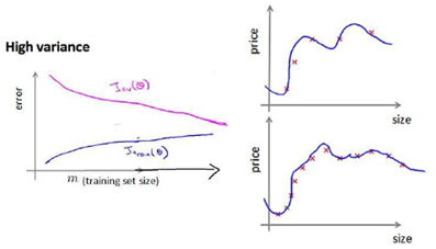
If a learning algorithm is suffering from high variance, getting more training data is likely to help.
Deciding What to Do Next Revisited
Our decision process can be broken down as follows:
Getting more training examples: Fixes high variance
Trying smaller sets of features: Fixes high variance
Adding features: Fixes high bias
Adding polynomial features: Fixes high bias
Decreasing: Fixes high bias
Increasing Fixes high variance
Diagnosing Neural Networks
- A neural network with fewer parameters is prone to underfitting. It is also computationally cheaper.
- A large neural network with more parameters is prone to overfitting. It is also computationally expensive. In this case you can use regularization(increase) to address the overfitting.
Using a single hidden layer is a good starting default. You can train your neural network on a number of hidden layers using your cross validation set. You can then select the one that performs best.
Model Complexity Effects:
- Low-order polynomials(low model complexity) have high bias and low variance. In this case, the model fits poorly consistently.
- Higher-order polynomials(high model complexity) fit the training data extremely well and the test data extremely poorly. These have low bias on the training data, but very high variance.
- In reality, we would want to choose a model somewhere in between, that can generalize well but also fits the data reasonably well.
Building a Spam Classifier
Prioritizing What to Work On
System Design Example:
Given a data set of emails, we could construct a vector for each email. Each entry in this vector represents a word. The vector normally contains 10,000 to 50,000 entries gathered by finding the most frequently used words in our data set. If a word is to be found in the email, we would assign its respective entry a 1, else if is not found, that entry would be a 0. Once we have all our x vectors ready, we train our algorithm and finally, we could use it to classify if an email is a spam or not.
So how could you spend your time to improve the accuracy of this classifier?
- Collect lots of dada (for example "honepot" project but doesn't always work)
- Develop sophisticated features(for example: using email header data in spam emails)
- Develop algorithms to process your input in difference ways(recognizing misspellings in spam).
It is difficulty to tell which of the options will be most helpful.
Error Analysis
The recommended approach to solving machine learning problems is to:
Start with a simple algorithm, implement it quickly, and test it early on your cross validation data.
Plot learning curves to decide if more data, more features, etc. are likely to help.
Manually examine the errors on examples in the cross validation set and try to spot a trend where most of the errors were made.
For example, assume that we have 500 emails and our algorithm misclassifies a 100 of them. We could manually analyze the 100 emails and categorize them based on what type of emials they are. We could then try to come up with new cues and features that would help us classify these 100 emials correctly. Hence, if most of our misclassified emails are those which try to steal passwords, then we could find some features that are particular to those emails and add them to our model. We could also see how classifying each word according to its root changes our error rate:
It is very important to get error results as a single, numerical value. Otherwise it is difficult to assess your algorithm's performance. For example if we use stemming, which is the process of treating the same word with different forms (fail/failing/failed) as one word (fail), and get a 3% error rate instead of 5%, then we should definitely add it to our model. However, if we try to distinguish between upper case and lower case letters and end up getting a 3.2% error rate instead of 3%, then we should avoid using this new feature. Hence, we should try new things, get a numerical value for our error rate, and based on our result decide whether we want to keep the new feature or not.
Support Vector Machines
Large Margin Classification
Optimization Objective
We are simplifying the logistic regression cost function by converting(交换) the sigmoid function into two straight lines, as shown here:
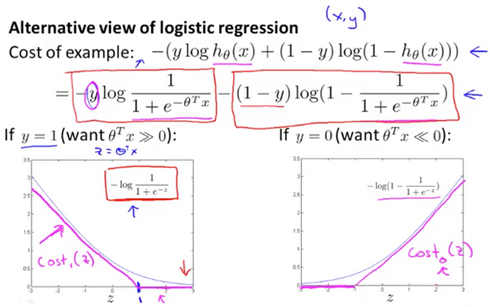
The following are two cost functions for support vector machines:

They both give the same value of if .
Hypothesis will predict:

Large Margin Intuition

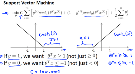
On the left plotted of z function for positive examples, on the right plotted z function, the z on the horizontal axis. If we have a positive example, we really want , and conversely if y is equal to zero, , this builds in an extra safety factor or safety margin factor into the support vector machine.
If C is very,very large, then when minimizing this optimization objective, we're going to be highly motivated to choose a value, so that this first term is euqal to zero.

So we saw alreadly that whenever we have a training example with a label of y=1, we want to make that first term to zero, we need . If y=0, we need When we minimize this as a function of the parameter , we get a interesting decision boundary.

There have many a different straight lines,but The support Vector Machines will instead choose the black boundary. The black line seems like a more robust separator, it does a better job of separating the positive and negative examples. And mathematically, the black decision boundary has a larger distance. That distance is called the margin. 因此支持向量机有时被称为大间距分类器。

当C的值非常大的时候,并且有一个异常点,则会选择粉色的线,这是不明智的。如果你将C设置的不要太大,则你最终会得到这黑线。
C较大时,相当于 较小,可能会导致过拟合,高方差。
C较小时,相当于 较大,可能会导致低拟合,高偏差。
Mathematics Behind Large Margin Classification
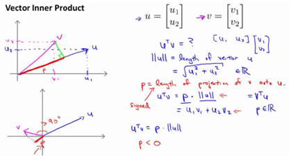
表示u的范数,即u的长度,即向量u的欧几里得长度。
使用向量内积的性质来理解支持向量机中的目标函数,当C很大时,目标函数可做一些简化得到如下的表达式
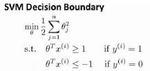
令得到两个特征
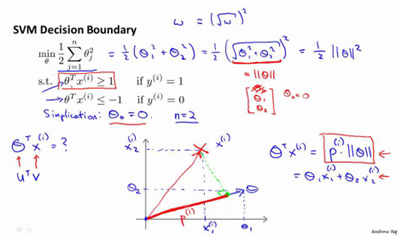
支持向量机做的全部事情,就是极小化参数向量范数的平方,或者说长度的平方。
因为 ,将其写入目标函数,得到
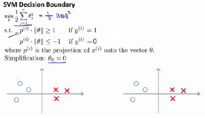
根据 画出边界,参数事实上是和决策界是90度正交的。
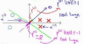
如果边界函数如上图所示,那么将会是非常小的数,当特别小,要满足那就意味着的范数非常大,因此,着看起来不像是一个好的参数向量的选择。
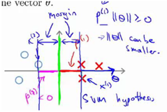
当变大了,仍然要满足那就意味着的范数变小了。因此,如果我们想令的范数变小,从而令范数的平方变小,就能让支持向量机选择下面的决策界,这就是支持向量机如何能有效地产生大间距分类的原因。
Kernels
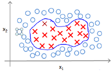
为了获得上图的判定边界,我们的模型可以是

我们可以用一系列的新特征f来替换模型中的每一项。例如令:

给定一个训练实例x,我们利用x的各个特征与我们预先选定的地标(landarks),,的近似程度来选取新的特征,
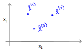
例如

其中

为实例x中所有的特征与地标之间的距离的和。上例中的就是核函数,具体而言,这是一个高斯核函数(Gaussian kernel)。注:这个函数与正态分布没有什么实际上的关系,只是看上去像而已。
如果一个训练实例x与地标L之间的距离近似于0,则新特征f近似于1,如果训练实例x与地标L之间距离较远,则f近似于0.
假设我们的训练实例含有两个特征,给定地标与不同的值
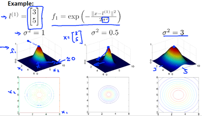
图中水平面的坐标为而垂直坐标轴代表f。可以看出,只有x与重合时f才具有最大值。随着x的改变f值改变的速率受到的控制。

如何选择地标?
通常是根据训练集的数量选择地标的数量,即如果训练集中有m个实例,则我们选取m个地标,并且令:

这样做的好处在于:现在我们得到的新特征是建立在原有特征与训练集中所有其他特征之间距离的基础之上的,即:
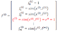
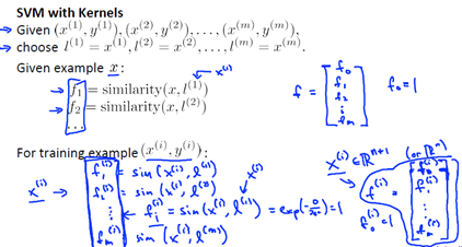
下面将核函数运用到支持向量机中,修改我们的支持向量机假设为:
给定x,计算新特征f,当时,预测y=1,否则反之。相应的修改代价函数为:

支持向量机也可以不使用核函数,不使用核函数又称为线性核函数(linear kernel),当我们不采用非常复杂的函数,或者我们的训练集特征非常多而实例非常少的时候,可以采用这种不带核函数的支持向量机。
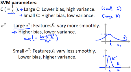
下面是支持向量机的两个参数C和的影响:
C=1/
C较大时,相当于较小,可能会导致过拟合,高方差
C较小时,相当于较大,可能会导致低拟合,高偏差
较大时,可能会导致低方差,高偏差
较小时,可能会导致低偏差,高方差。
When to choose between a linear kernel and a gaussian kernel?
Note:When using the Gaussian kernel, it is important to perform feature scaling beforehand.
The kernels that you choose must satisfy a technical condition called "Mercer's Theorem" to make sure SVM packages' optimizations run correctly and do not diverge.
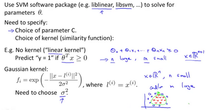

Logistic regression vs Source Vector Machines
- If n(特征) is large relative to m(样本)(n=10,000 m=10-1000),use logistic regression, or SVM without a kernel("linear kernel")
- if n is small and m is intermediate(n=1-1000,m=10-10,000),use SVM with Gaussian kernel
- If n is small and m is large (n=1-1000,m=50000+), Create/add more fearures, then use logistic regression or SVM without a kernel
Neural networks are likely to work well for most of these setttings, but may be slower to train.
Unsupervised Learning
Clustering
Introduction
Unsupervised learning is the class of problem solving where when given a set of data with no labels, find structure in the dataset.
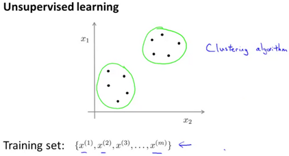
Clustering is good for problems like:
- Market segmentation(Create groups for your potential customers)
- Social Network analysis(analyze groups of friends)
- Organize computing clusters(arrange severs in idea locations to one another)
- Astronomical (天体) data analysis(Understand groupings of stars)
K-Means Algorithms
This is a clustering algorithm.
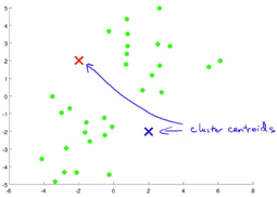
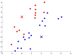
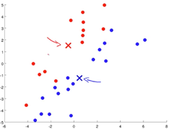
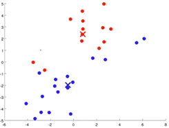
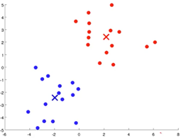
- Randomly initialize your cluster centroids
- Cluster assignment step:Assign each example to a cluster centroid based on distance.
- Move centroid step:Take the centroids,move them to the average of all the assigned examples.
- Iterate through step 2 and step 3 until convergence.
1 2
3 4
5
Formal Definition
Input:
- K(number of clusters)
- Training set{}
Randomly initialize K cluster centroids
Repeat{
- Cluster Assignment Step
For i=1 to m,:=index(from 1 to K) of cluster centroid closest to
- Move Centroid Step
For k=1 to K, := average(mean) of points assigned to cluster k
}
If there are clusters with no points assigned to it, it is common practice to remove that cluster. Alternatively, one may reinitialize the algorithm with new cluster centroids.
Optimization Objective
The K-Means cost function (optimization objective) is defined here:
=index of cluster(1,2,…,K) to which example is currently assigned cluster centroid k ()
=cluster centroid of cluster to which example has been assigned

Random Initialization
How do you initialize the cluster centroids?
- Pick a number of clusters less then the number of examples you have
Should have K<m
- Randomly pick K training examples
- Set equal to these K examples
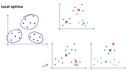
The K-Means algorithm may end up in local optima. The way to get aroud this is to run K-Mean multiple times with multiple random initializations. A typical number of times to run K-Means is 50-1000 times. Compute the cost function J and pick the clustering that gives the lowest cost.
Choosing the Number of Clusters
Choosing the number of clusters K in K-means is a non trivial problem as clusters may or may not be intuitive. Usually , it is still a manual step where an individual picks the number of clusters by looking at a plot.
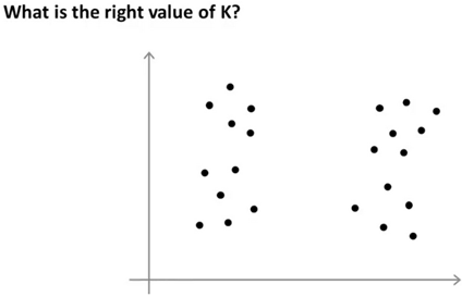
Are there 2,3,or 4 clusters? It's ambiguous
Elbow Method
- Run K-Means with varying number of cluster.(1 cluster, the 2 cluster, the 3…. So on and so on)
- Ends up with a curve showing how distortion decreases as the number of clusters increases.
- Usually the 'elbow' is not clearly defined
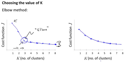
Usually K-Means is downstream purpose specific. For example, when calculating clusters for market segmentation, if we are selling T-Shirts, perhaps it is more useful to have predefined clusters "Small, Medium, Large" or "Extra Small, Medium, Large, Extra Large" size.
Dimensionality Reduction
Motivation
Data Compression
There are two primary reasons to perform dimensionality reduction. One of them is data compression, and the other is that dimensionality reduction can increase performance of our learning algorithm.
Given a two features like length in inches and centemeters, with slight roundoff erro, there is a lot of redundancy(冗余). It would be useful to convert a 2D plot into a 1D vector.
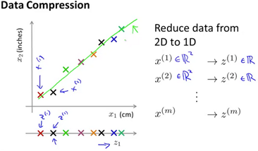
Before, we needed two numbers to represent an example. After compression, only one number is necessary to represent the example.
The typical example of dimensionality reduction is from 1000D to 100D.
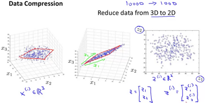
Visualization
Dimensionality Reduction also helps us visualize the data better. Suppose we have the following dataset:
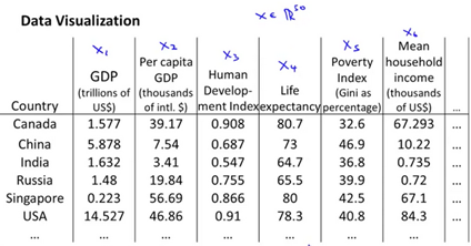
We want to reduce the features to a two or three dimensional vector in order to better understand the data, rather than attempt to plot a 50 dimension table.

Principal Component Analysis
Principal Component Analysis Problem Formulation
PCA is the most popular algorithm to perform dimensionality reduction.
- Find a lower dimensional surface such that the sum of squares error(projection error) is minimized.
- Standard practice is to perform feature scalining and mean normalization before scaling the data.
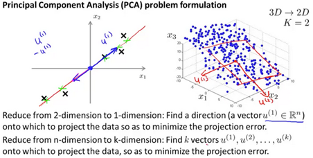
PCA is not linear regression

In linear regression, we are minimizing the point and the value predicted b the hypothesis.
In PCA, we are minimizing the distance between the point and the line.
Principal Component Analysis Algorithm
- Data preprocessing step:
- Given your training set
- Perform feature scaling and mean normalization

- Replace each with .
- If different feature on different scale,(e.g size of house, number of bedrooms) scale features to have compareble range of values.

- PCA algorithm
- Reduce data from n-dimensions to k-dimensions
- Compute the "covariance matrix"(协方差矩阵):
- (it is unfortunate that the Sigma value is used, do not confuse with summation)

- Compute the 'eigenvectors'(特征向量) of matrix
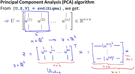
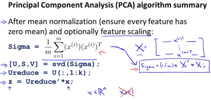
Applying PCA
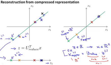
Reconstruction(重建) from compressed Representation(表示)
After compression, how do we go back to the higher dimensional state?
Choosing the Number of Principal Components
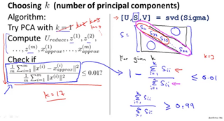
In the PCA algorithm, how do we choose the value for K? How do we choose the number of principal components?
Recall that PCA tries to minimize the average squared projection error

Also, the total variation in the data is defined as

Typically choose k to be the smallest value such that
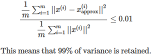
Vary the percentage between 95-99 percent, depending on your application and requirements.
This is how to calculate the variance using the svd(Sigma) function return values:
Advice for Applying PCA
PCA can be applied to reduce your training set dimensions before feeding the resulting training set to a learning alogritm.
Only run PCA on the training set. Do not run PCA on the cross validation and test sets.
One bad use of PCA is to prevent overfitting. Use regularization instead. PCA throws away some information without knowing what the correspinding values of y are.
Do not unnecessarily run PCA. It is valid to run your learning algorithms using the raw data and only when that fails, implement PCA.
Anomaly Detection
Density Estimation(密度估计)
Problem Motivation
Imagine being a manufacturor of aircraft engines. Measure heat generated, vibration intensity, etc. You know have a dataset of these features which you can plot. Anomoly detection would be determining if a new aircraft engine is anomolous in relation to the previously measured engine features.
Given a dataset anomalous? Check if for given test set.
Some useful cases include fraud detection, manufacturing, monitoring computers in a data center,etc.
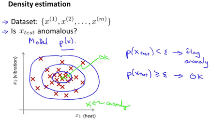
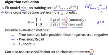
Suppose the anomaly detection system flags x as anomalous whenever . It is flagging too many things as anomalous that are not actually so. The corrective step in this case would be to decrease the value of .
Gaussian Distribution
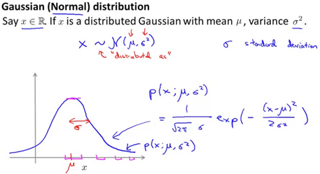
The Gaussian Distribution(Normal Distribution), where , has mean u and variance :

(The tilde(波浪号) means "distributed as"(服从什么分布), Script 'N' stands for normal distribution.

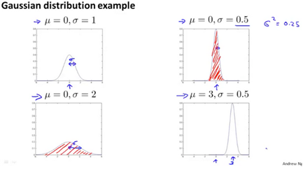
Red shaded area is equal to 1.
To calculate the average u and variance we use the following formulae:

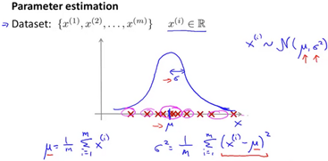
Algorithm
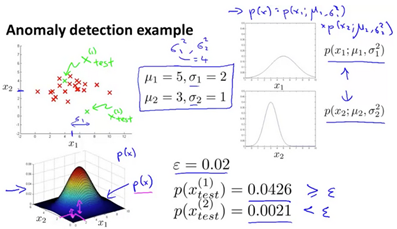
Algorithm for density estimation. Given a training set where each example is

Where

And so on.
More conscicely, this algorithm can be written as:

The capital is the product symbol, it is similar to the function except rather than adding, it performs multiplication.
- Choose features that you think might be indicative of anomalous examples.
- Fit parameters
- Given new example x, compute p(x). The example is an anomaly if .
Building an Anomaly Detection System
Developing and Evaluating an Anomaly Detection System
The importance of real-number evalution, when developing a learning algorithm, learning decisions is much easier if we have a way of evaluating our learning algorithm. Assume we have some labeled data of anomalous and non-anomalous examples.(y=0 if normal and y=1 as anomalous)
Training set: (assume that the training set is normal and not anomalous)
Cross validation set:

Test set:

The following would be a recommended split of training sets and cross validation sets for an aircraft engine monitoring examplel:
One can evaluate the algorithm by using precision and recall, of the score.
Anomaly Detection vs. Supervised Learning
Anomaly detection can be used if there are a very small number of positive examples(y=1, a range between zero and twenty is common). Anomaly detection should also have a large number of negative (y=0) examples. Anomalies should have many types, it's hard for any algorithm to learn what anomalies look like, as future anomalies may look nothing like what we have seen so far.
- Fraud Detection
- Manufacturing(eg aircraft engines)
- Monitoring machines in a data center
Supervised learning should be used when there are a large number of positive and negative ezamples. There are enough positive examples for the algorithm to get a sense of what positive example are like. Future positive examples are likely to be similar to the ones in the training set.
- Email/Spam classification
- Weather prediction(sunny/rainy/etc)
- Cancer classification
Choosing What Features to Use
One thing that we have done was plotting the features to see if the features fall into a normal(gaussian) distribution. Given a dataset that does not look gaussian, it might be useful to transform the features to look more gaussian. There are multiple different functions one can play with to make the data look more gaussian.
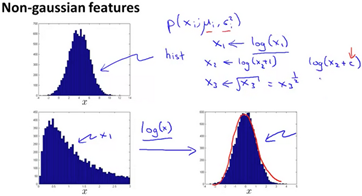
Error analysis for anomaly detection, we want p(x) to be large for normal examples and p(x) to be small for anomallous examples.
How do we fix the common problem where p(x) is comparable for both normal and anomalous examples? This is still a manual process, look at the anomalous examples and distinguish features that make the irregular exmaple anomalous.
Choose features that might take on unusually large or small values in the event of an anomaly.
Multivariate Gaussian Distribution
Algorithm
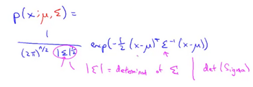
Multivariate Gaussian Distribution can be usefull if there are correlation between the features that need to be accounted for when when determining anomalies.
It may be useful to not model separately. Model all in one go. Parameters are .

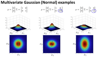
Here are some examples of multivariate gaussian examples with varying sigma:
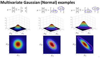
To perform parameter fitting, plug in the following formula:

Recomender Systems
Predicting Movie Ratings
Problem Forumulation
Imagine you are a company that sells or rents out movies. You allow users to rate different movies from zero to five stars. You have a matrix of users, their sparsely populated rated movies, and you want to find out what they would also rate similarly according to existing data.
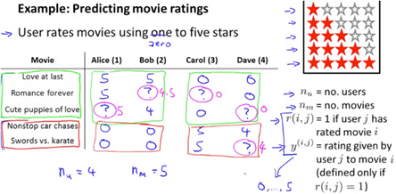
Content Based Recommemdations
If the movies have features associated to the movie, they can be represented with a feature vector.
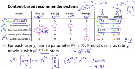
To learn refer to the followoing problem formulations:

TO learn :

Gradient Descent:

Collaborative Filtering(协同过滤)
Collaborative Filtering Algorithm
This algorithm learns what features to use for an existing data set. It can be very difficult to determine how 'romantic' a movie is, or how much 'action' a movie has. Suppose we have a data set where we do not know the features of our movies.
The assumption here is that users pre-specify what genres(类型) of movies they like.
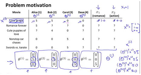
Given to learn

Given to learn :

Minimize and
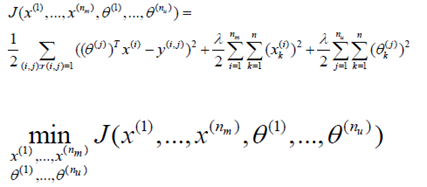

Initialize and to random small values.
Minimize J using gradient descent (or an advanced optimization algorithm).
For a user with parameters and a movie with (learned) features x predict a star rating of
Low Rank Matrix Factorization
Vectorization: Low Rank Matrix Factorization
The vectorized implementation for the recomender system can be visualized as the following:
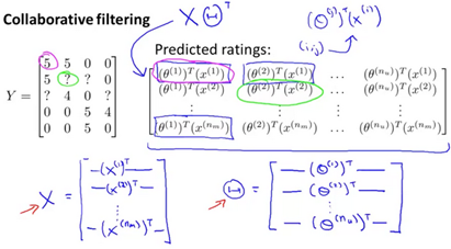
Movies can be related if the feature vectors between the movies are small.
Implementational Detail: Mean Normalization
For users who have not rated any movies, the only term that effects the user is the regularization term
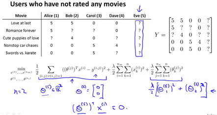
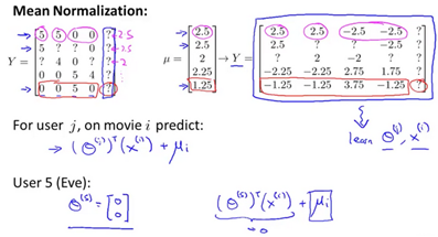
This does not help us perform reccomendations as the value of all predicted stars will be 0 for the user who haw not rated any movies. One way to address this is to apply mean normalization to the input data and pretend the normalized data is the new data to perform prediction with.
This allows us to perform reccomendations even though a user has not rated any movies, because we have the average rating of a movie based on all users.
Large Scale Machine Learning
Gradient Descent with Large Datasets
Learning With Large Datasets
One of the best ways to get a high performance machine learning system si to supply a lot of data into a low bias(overfitting) learning algorithm. The gradient descent algorithm can run very slowly if the training set is large, because a summation needs to be performed across all training examples to perform one step of gradient descent.
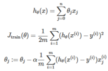
- What if m were 100,000,000? becomes very expensive.
- Could we do a sanity check by running gradient descent with 1000 randomly selected examples?
One way to verify this is to plot a learning curve for a range of values of m (say 100,1000,1000) and verify that the alogrithm has high variance (overfitting)
Stochastic Gradient Descent
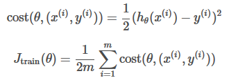
Rather than running gradient descent on the entire training set, one can run gradient descent on one training set at a time. The following is the Stochastic Gradient Descent algorithm:
Advanced Topics
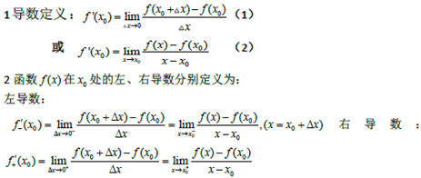
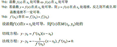
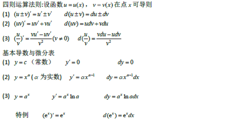
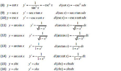
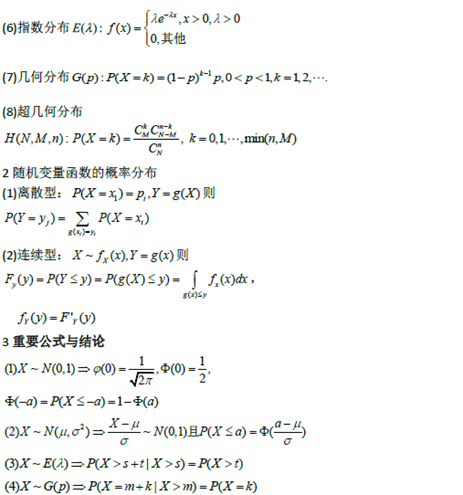
附:常用的数学公式
一元函数微分学
|
内容 |
对应公式、定理、概念 |
|
导数和微分的概念左右导数 导数的几何意义和物理意义 |
|
|
函数的可导性与连续性之间的关系,平面曲线的切线和法线 |
|
|
导数和微分的四则运算,初等函数的导数 |
|
|
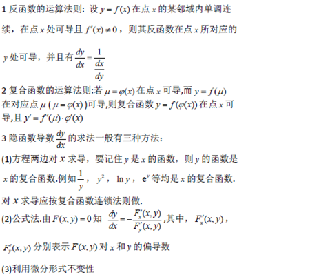
复合函数,反函数,隐函数以及参数方程所确定的函数的微分法 |
|
|
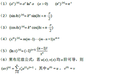
高阶导数,一阶微分形式的不变形 |
|
|
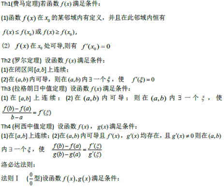
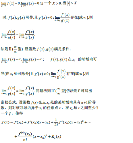
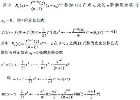
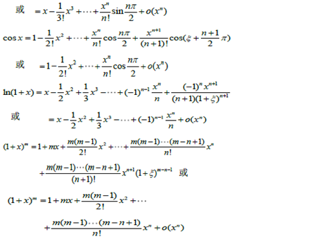
微分中值定理,必达法则,泰勒公式 |
|
|
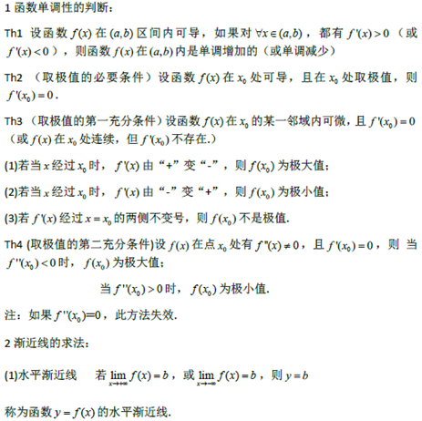
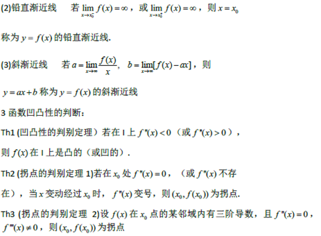
函数单调性的判别,函数的极值,函数的图形凸凹性,拐点及渐进性,用函数图形描绘函数最大值和最小值 |
|
|
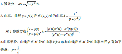
弧微分,曲率的概念,曲率半径 |
|
随机事件和概率
|
内容 |
对应概念,定理,公式 |
|
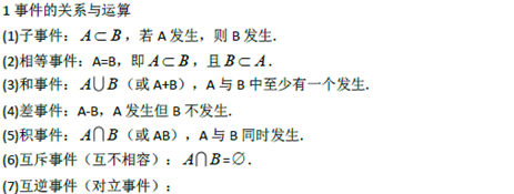
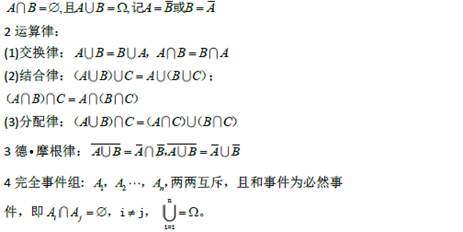
随机事件与样本空间,事件的关系与运算,完全事件组 |
|
|
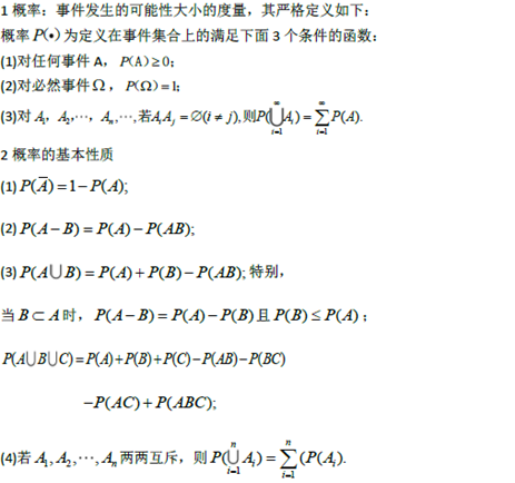
概率的概念,概率的基本性质,古典概率,几何型概率 |
|
|
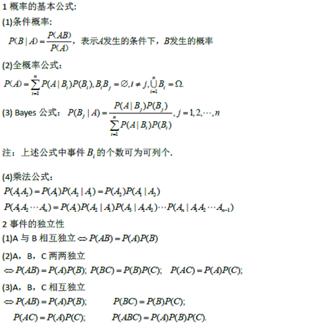
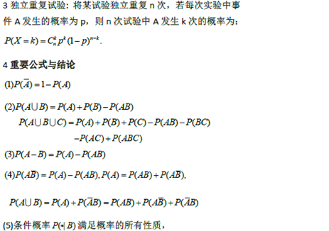
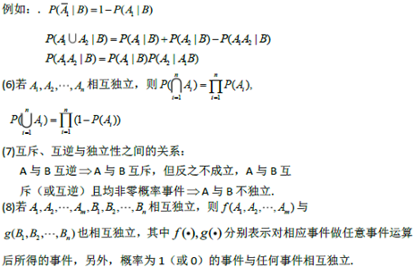
概率的基本公式,事件的独立性,独立重复试验 |
|
随机变量及其概率分布
|
内容 |
对应公式,概念,定理 |
|
随机变量,随机变量的分布函数的概念及其性质 |
|
|
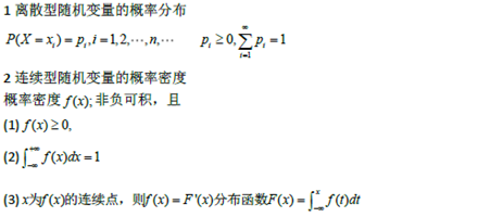
离散型随机变量的概率分布,连续型随机变量的概率密度性质 |
|
|
常见随机变量的概率分布,随机变量函数的概率分布 |
|
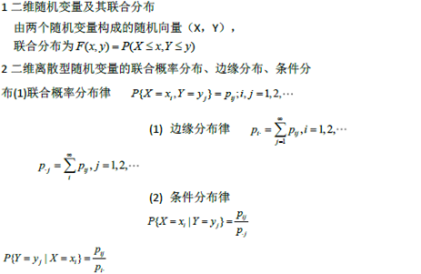
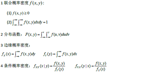
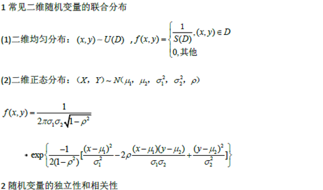
多维随机变量及其分布
|
内容 |
对应公式、概念、定理 |
|
多维随机变量及其分布,二维离散型随机变量的概率分布、边缘分布和条件分布 |
|
|
二位连续性随机变量的概率密度、边缘概率密度和条件密度 |
|
|
随机变量的独立性和不相关性,常用二维随机变量的分布 |
|
|
两个及两个以上随机变量简单函数的分布 |
|
随机变量的数字特征
|
内容 |
对应概念、定义、定理、公式 |
|
随机变量的数学期望(均值)、方差和标准差及其性质 |
|
|
随机变量函数的数学期望,矩、协方差,相关系数的数字特征 |
|
大数定理和中心极限定理
|
内容 |
对应公式、概念、定理 |
|
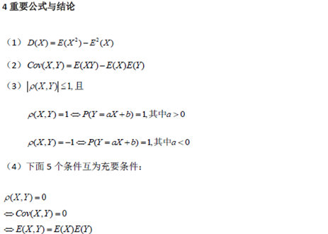
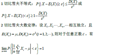
切比雪夫不等式,切比雪夫大数定律 |
|
|
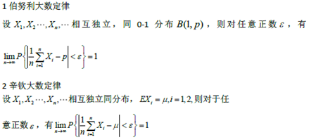
伯努利大数定律,辛钦大数定律 |
|
|
拉普斯定理 |
|
数理统计的基本概念
|
内容 |
对应公式、概念、定理 |
|
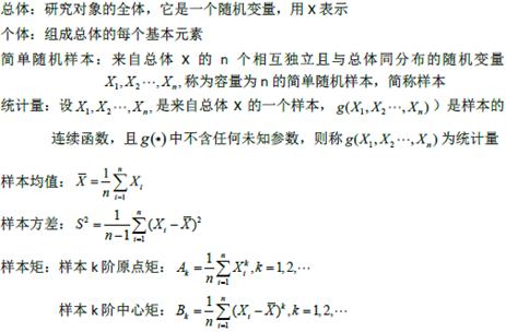
总体,个体,简单随机样本,统计量,样本均值,样本方差和样本矩 |
|
|
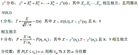
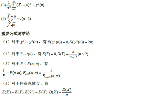
分布,t分布,F分布,分位数 |
|
|
正态总体的常用样本分布 |
|
参数估计
|
内容 |
对应公式、概念、定理 |
|
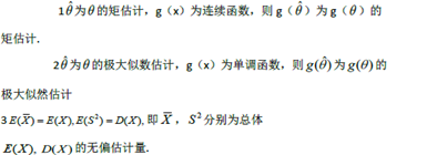
点估计的概念,估计量与估计值,矩估计法,最大似然估计法 |
|
|
估计量的评选标准区间估计的概念 |
|
|
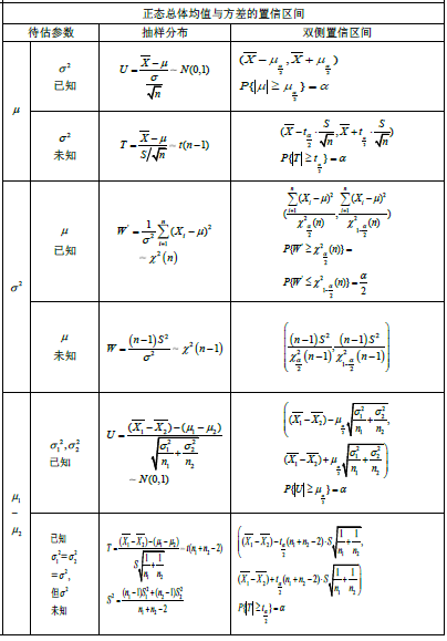
单个正态总体的均值和方差的区间估计,两个正态总体的均值差和方差比的区间估计 |
|
假设检验
|
内容 |
对应公式、概念、定理 |
|
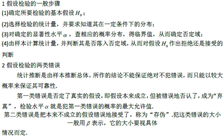
显著性检验、假设检验的两类错误 |
|
|
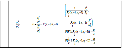
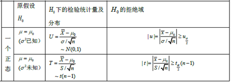
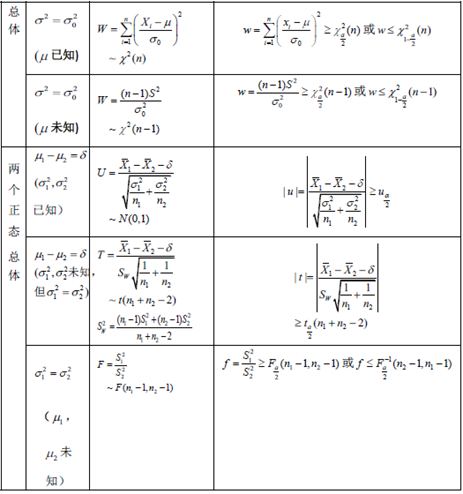
单个及两个正态总体的均值和方差的假设检查 |
|
Course Machine Learning Note的更多相关文章
- Machine Learning Note Phase 1( Done!)
Machine Learning 这是第一份机器学习笔记,创建于2019年7月26日,完成于2019年8月2日. 该笔记包括如下部分: 引言(Introduction) 单变量线性回归(Linear ...
- Machine Learning Note - Note 1
I am working on the Andrew Ng's course on Machine Learing. I have a question on the week2 session. I ...
- Machine Learning Note
[Andrew Ng NIPS2016演讲]<Nuts and Bolts of Applying Deep Learning (Andrew Ng) 中文详解:https://mp.weixi ...
- How do I learn machine learning?
https://www.quora.com/How-do-I-learn-machine-learning-1?redirected_qid=6578644 How Can I Learn X? ...
- Note for video Machine Learning and Data Mining——Linear Model
Here is the note for lecture three. the linear model Linear model is a basic and important model in ...
- 【Machine Learning】Python开发工具:Anaconda+Sublime
Python开发工具:Anaconda+Sublime 作者:白宁超 2016年12月23日21:24:51 摘要:随着机器学习和深度学习的热潮,各种图书层出不穷.然而多数是基础理论知识介绍,缺乏实现 ...
- [Python & Machine Learning] 学习笔记之scikit-learn机器学习库
1. scikit-learn介绍 scikit-learn是Python的一个开源机器学习模块,它建立在NumPy,SciPy和matplotlib模块之上.值得一提的是,scikit-learn最 ...
- Kernel Functions for Machine Learning Applications
In recent years, Kernel methods have received major attention, particularly due to the increased pop ...
- Machine Learning Algorithms Study Notes(2)--Supervised Learning
Machine Learning Algorithms Study Notes 高雪松 @雪松Cedro Microsoft MVP 本系列文章是Andrew Ng 在斯坦福的机器学习课程 CS 22 ...
随机推荐
- vue.js2.0实战填坑记录
访https://github.com/bailicangdu/vue2-elm的PC商城 在创建的 router 对象中,如果不配置 mode,就会使用默认的 hash 模式,该模式下会将路径格式化 ...
- xml和TreeView
1.TreeView代码代码: private void Form1_Load(object sender, EventArgs e) {<br> //代码为TreeView添加子项 tr ...
- IDEA JavaSE环境配置
需指定JDK路径: File -> Project Structure -> Project -> Project SDK -> New -> 选择JDK所在的根目录
- linux学习笔记汇总
linux 文件系统是采用级层树状的目录结构,采用"/"根目录的方式 目录结构: / 根目录 |---root: 存放root用户相关的文件 ...
- cp参数详解
-a 相当于pdr的意思 -d 若原文件为连接文件,则复制链接文件属性,而非文件本身 -f 强制复制,有重复时,不询问用户,而直接强制复制 -i 目标文件存在的话,先询问 -p 与文件的属性一起复制 ...
- Spring MVC系列[2]——参数传递及重定向
1.目录结构 2.代码 <?xml version="1.0" encoding="UTF-8"?> <web-app version=&qu ...
- EJB2.0版本的HelloWorld
EJB2.0版本的HelloWorld 虽然EJB3.1已经出来了,可是EJB2.0的项目还需要维护啊.下面写个简单EJB2.0的HelloWorld程序,练练手. 环境: JBoss 4.0 ...
- UVA10917 A walk trough the Forest (最短路,dp)
求出家到其他点的最短路径,题目的条件变成了u->v不是回头路等价于d[u]>d[v]. 然后根据这个条件建DAG图,跑dp统计方案数,dp[u] = sum(dp[v]). #includ ...
- Solr版本安装部署指南
一.依赖包 1. JDK 1.6以上 2. solr-4.3.0.tgz 3. Tomcat或者jetty(注意,solr包中本身就含有jetty的启动相关内容):apache-tomcat-7 ...
- ping 不通。无法访问目标主机
台式机 使用无线网卡 又登录了VPN 有时候访问不了局域网内的主机 解决方案 添加路由即可 window+R 打开运行 输入cmd 然后输入 route add 10.16.1.89 10.13 ...

