Statistics in Python

Statistics in Python

Materials for the “Statistics in Python” euroscipy 2015 tutorial.

Requirements

• Standard scientific Python environment (numpy, scipy, matplotlib)
• Pandas
• Statsmodels
• Seaborn

To install Python and these dependencies, we recommend that you downloadAnaconda Python, or use Ubuntu’s package manager.

 

Why Python for statistics?

R is a language dedicated to statistics. Python is a general purpose language with statistics module. R has more statistical analysis features than Python, and specialized syntaxes. However, when it comes to building complex analysis pipelines that mix statistics with e.g. image analysis, text mining, or control of a physical experiment, the richness of Python is an invaluable asset.

---

Contents

• 1   Data representation and interaction
  • 1.1   Data as a table
  • 1.2   The panda data-frame
• 2   Hypothesis testing: comparing two groups
  • 2.1   Student’s t-test
  • 2.2   Paired tests: repeated measurements on the same indivuals
• 3   Linear models, multiple factors, and analysis of variance
  • 3.1   “formulas” to speficy statistical models in Python
  • 3.2   Multiple Regression: including multiple factors
  • 3.3   Post-hoc hypothesis testing: analysis of variance (ANOVA)
• 4   More visualization: seaborn for statistical exploration
• 5   Testing for interactions
• 6   Full examples

In this document, the Python prompts are represented with the sign “>>>”. To copy-paste code, you can click on the top right of the code blocks, to hide the prompts and the outputs.

 

1   Data representation and interaction

1.1   Data as a table

The setting that we consider for statistical analysis is that of multipleobservations or samples described by a set of different attributes or features. The data can than be seen as a 2D table, or matrix, with columns given the different attributes of the data, and rows the observations. For instance, the data contained in examples/brain_size.csv:

"";"Gender";"FSIQ";"VIQ";"PIQ";"Weight";"Height";"MRI_Count"

 

"1";"Female";133;132;124;"118";"64.5";816932

 

"2";"Male";140;150;124;".";"72.5";1001121

 

"3";"Male";139;123;150;"143";"73.3";1038437

 

"4";"Male";133;129;128;"172";"68.8";965353

 

"5";"Female";137;132;134;"147";"65.0";951545

 

1.2   The panda data-frame

We will store and manipulate this data in a pandas.DataFrame, from the pandas module. It is the Python equivalent of the spreadsheet table. It is different from a 2D numpy array as it has named columns, can contained a mixture of different data types by column, and has elaborate selection and pivotal mechanisms.

1.2.1   Creating dataframes: reading data files or converting arrays

Separator

It is a CSV file, but the separator is ”;”

Reading from a CSV file: Using the above CSV file that gives observations of brain size and weight and IQ (Willerman et al. 1991), the data are a mixture of numerical and categorical values:

>>>

>>> import pandas

 

>>> data = pandas.read_csv('examples/brain_size.csv', sep=';', na_values=".")

 

>>> data

 

    Unnamed: 0  Gender  FSIQ  VIQ  PIQ  Weight  Height  MRI_Count

 

0            1  Female   133  132  124     118    64.5     816932

 

1            2    Male   140  150  124     NaN    72.5    1001121

 

2            3    Male   139  123  150     143    73.3    1038437

 

3            4    Male   133  129  128     172    68.8     965353

 

4            5  Female   137  132  134     147    65.0     951545

 

...

 

Warning

Missing values

The weight of the second individual is missing in the CSV file. If we don’t specify the missing value (NA = not available) marker, we will not be able to do statistical analysis.

 

Creating from arrays:: data-frames can also be seen as a dictionary of 1D ‘series’, eg arrays or lists. If we have 3 numpy arrays:

>>>

>>> import numpy as np

 

>>> t = np.linspace(-6, 6, 20)

 

>>> sin_t = np.sin(t)

 

>>> cos_t = np.cos(t)

 

We can expose them as a pandas dataframe:

>>>

>>> pandas.DataFrame({'t': t, 'sin': sin_t, 'cos': cos_t})

 

         cos       sin         t

 

0   0.960170  0.279415 -6.000000

 

1   0.609977  0.792419 -5.368421

 

2   0.024451  0.999701 -4.736842

 

3  -0.570509  0.821291 -4.105263

 

4  -0.945363  0.326021 -3.473684

 

5  -0.955488 -0.295030 -2.842105

 

6  -0.596979 -0.802257 -2.210526

 

7  -0.008151 -0.999967 -1.578947

 

8   0.583822 -0.811882 -0.947368

 

...

 

 

Other inputs: pandas can input data from SQL, excel files, or other formats. See the pandas documentation.

 

1.2.2   Manipulating data

data is a pandas dataframe, that resembles R’s dataframe:

>>>

>>> data.shape    # 40 rows and 8 columns

 

(40, 8)

 

 

>>> data.columns  # It has columns

 

Index([u'Unnamed: 0', u'Gender', u'FSIQ', u'VIQ', u'PIQ', u'Weight', u'Height', u'MRI_Count'], dtype='object')

 

 

>>> print data['Gender']  # Columns can be addressed by name

 

0     Female

 

1       Male

 

2       Male

 

3       Male

 

4     Female

 

...

 

 

>>> # Simpler selector

 

>>> data[data['Gender'] == 'Female']['VIQ'].mean()

 

109.45

 

Note

For a quick view on a large dataframe, use its describe method:pandas.DataFrame.describe().

groupby: splitting a dataframe on values of categorical variables:

>>>

>>> groupby_gender = data.groupby('Gender')

 

>>> for gender, value in groupby_gender['VIQ']:

 

...     print gender, value.mean()

 

Female 109.45

 

Male 115.25

 

groupby_gender is a powerfull object that exposes many operations on the resulting group of dataframes:

>>>

>>> groupby_gender.mean()

 

        Unnamed: 0   FSIQ     VIQ     PIQ      Weight     Height  MRI_Count

 

Gender

 

Female       19.65  111.9  109.45  110.45  137.200000  65.765000   862654.6

 

Male         21.35  115.0  115.25  111.60  166.444444  71.431579   954855.4

 

Use tab-completion on groupby_gender to find more. Other common grouping functions are median, count (useful for checking to see the amount of missing values in different subsets) or sum. Groupby evaluation is lazy, no work is done until an aggregation function is applied.

 

Exercise

• What is the mean value for VIQ for the full population?

• How many males/females were included in this study?

  Hint use ‘tab completion’ to find out the methods that can be called, instead of ‘mean’ in the above example.

• What is the average value of MRI counts expressed in log units, for males and females?

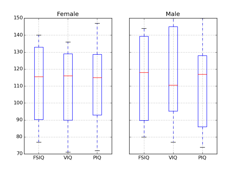
Note

groupby_gender.boxplot is used for the plots above (see this example).

 

1.2.3   Plotting data

Pandas comes with some plotting tools (that use matplotlib behind the scene) to display statistics of the data in dataframes:

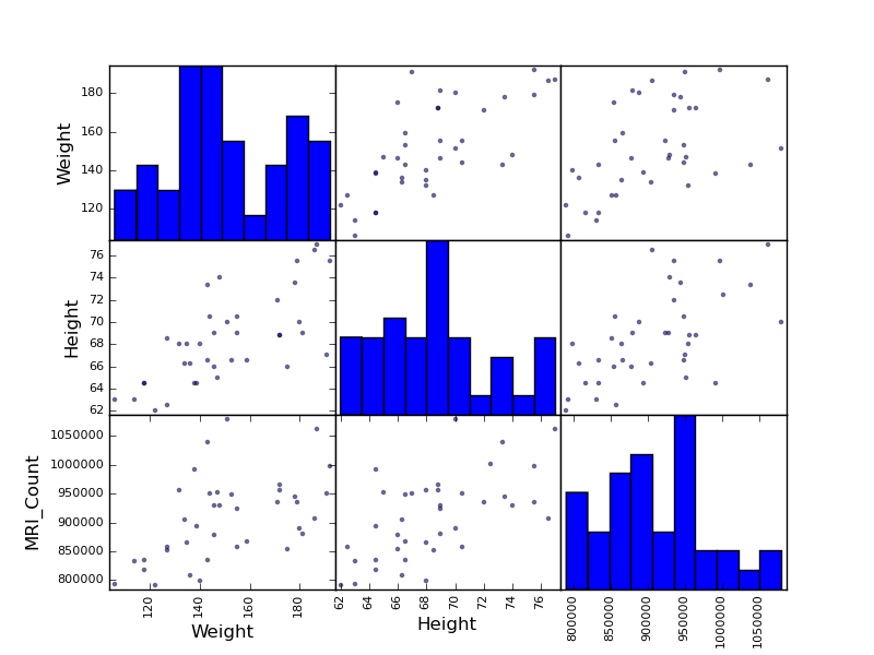
Scatter matrices:

>>>

>>> from pandas.tools import plotting

 

>>> plotting.scatter_matrix(data[['Weight', 'Height', 'MRI_Count']])

 

>>>

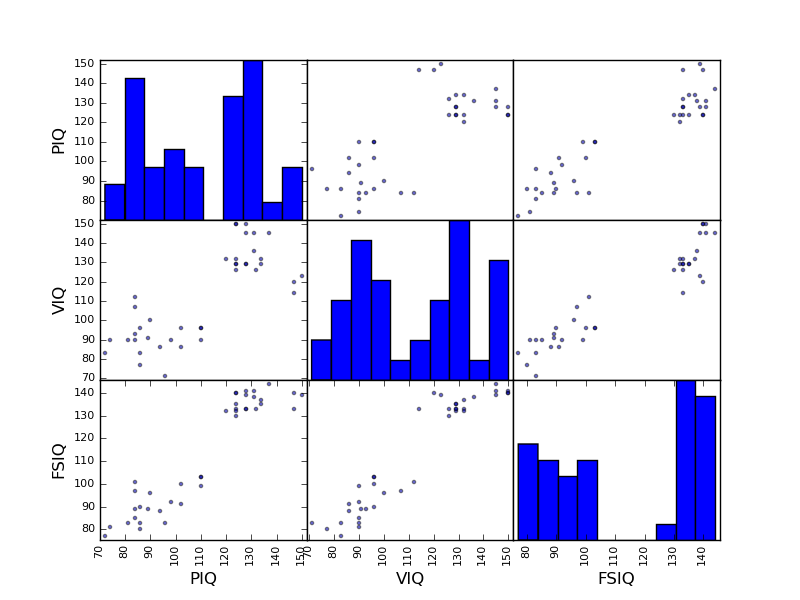
>>> plotting.scatter_matrix(data[['PIQ', 'VIQ', 'FSIQ']])

 

Two populations

The IQ metrics are bimodal, as if there are 2 sub-populations.

Exercise

Plot the scatter matrix for males only, and for females only. Do you think that the 2 sub-populations correspond to gender?

 

2   Hypothesis testing: comparing two groups

For simple statistical tests, we will use the stats sub-module of scipy:

>>>

>>> from scipy import stats

 

See also

Scipy is a vast library. For a tutorial covering the whole scope of scipy, see http://scipy-lectures.github.io/

2.1   Student’s t-test

2.1.1   1-sample t-test

scipy.stats.ttest_1samp() tests if observations are drawn from a Gaussian distributions of given population mean. It returns the T statistic, and the p-value (see the function’s help):

>>>

>>> stats.ttest_1samp(data['VIQ'], 0)

 

(array(30.088099970...), 1.32891964...e-28)

 

With a p-value of 10^-28 we can claim that the population mean for the IQ (VIQ measure) is not 0.

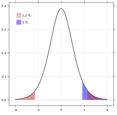
Exercise

Is the test performed above one-sided or two-sided? Which one should we use, and what is the corresponding p-value?

2.1.2   2-sample t-test

We have seen above that the mean VIQ in the male and female populations were different. To test if this is significant, we do a 2-sample t-test withscipy.stats.ttest_ind():

>>>

>>> female_viq = data[data['Gender'] == 'Female']['VIQ']

 

>>> male_viq = data[data['Gender'] == 'Male']['VIQ']

 

>>> stats.ttest_ind(female_viq, male_viq)

 

(array(-0.77261617232...), 0.4445287677858...)

 

2.2   Paired tests: repeated measurements on the same indivuals

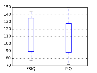
PIQ, VIQ, and FSIQ give 3 measures of IQ. Let us test if FISQ and PIQ are significantly different. We need to use a 2 sample test:

>>>

>>> stats.ttest_ind(data['FSIQ'], data['PIQ'])

 

(array(0.46563759638...), 0.64277250...)

 

The problem with this approach is that it forgets that there are links between observations: FSIQ and PIQ are measured on the same individuals. Thus the variance due to inter-subject variability is confounding, and can be removed, using a “paired test”, or “repeated measures test”:

>>>

>>> stats.ttest_rel(data['FSIQ'], data['PIQ'])

 

(array(1.784201940...), 0.082172638183...)

 

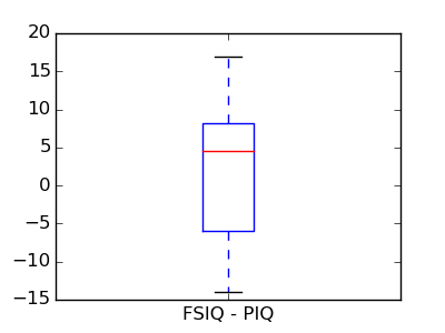
This is equivalent to a 1-sample test on the difference:

>>>

>>> stats.ttest_1samp(data['FSIQ'] - data['PIQ'], 0)

 

(array(1.784201940...), 0.082172638...)

 

 

T-tests assume Gaussian errors. We can use aWilcoxon signed-rank test, that relaxes this assumption:

>>>

>>> stats.wilcoxon(data['FSIQ'], data['PIQ'])

 

(274.5, 0.106594927...)

 

Note

The corresponding test in the non paired case is the Mann–Whitney U test, scipy.stats.mannwhitneyu().

Exercice

• Test the difference between weights in males and females.
• Use non parametric statistics to test the difference between VIQ in males and females.

 

3   Linear models, multiple factors, and analysis of variance

3.1   “formulas” to speficy statistical models in Python

3.1.1   A simple linear regression

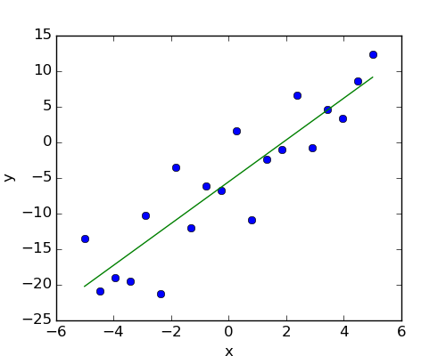
Given two set of observations, x and y, we want to test the hypothesis that y is a linear function of x. In other terms:

where e is observation noise. We will use the statmodels module to:

1. Fit a linear model. We will use the simplest strategy, ordinary least squares (OLS).
2. Test that coef is non zero.

 

First, we generate simulated data according to the model:

>>>

>>> import numpy as np

 

>>> x = np.linspace(-5, 5, 20)

 

>>> np.random.seed(1)

 

>>> # normal distributed noise

 

>>> y = -5 + 3*x + 4 * np.random.normal(size=x.shape)

 

>>> # Create a data frame containing all the relevant variables

 

>>> data = pandas.DataFrame({'x': x, 'y': y})

 

“formulas” for statistics in Python

See the statsmodels documentation

 

Then we specify an OLS model and fit it:

>>>

>>> from statsmodels.formula.api import ols

 

>>> model = ols("y ~ x", data).fit()

 

We can inspect the various statistics derived from the fit:

>>>

>>> print(model.summary())

 

                            OLS Regression Results

 

==============================================================================

 

Dep. Variable:                      y   R-squared:                       0.804

 

Model:                            OLS   Adj. R-squared:                  0.794

 

Method:                 Least Squares   F-statistic:                     74.03

 

Date:                ...                Prob (F-statistic):           8.56e-08

 

Time:                        ...        Log-Likelihood:                -57.988

 

No. Observations:                  20   AIC:                             120.0

 

Df Residuals:                      18   BIC:                             122.0

 

Df Model:                           1

 

==============================================================================

 

                 coef    std err          t      P>|t|      [95.0% Conf. Int.]

 

------------------------------------------------------------------------------

 

Intercept     -5.5335      1.036     -5.342      0.000        -7.710    -3.357

 

x              2.9369      0.341      8.604      0.000         2.220     3.654

 

==============================================================================

 

Omnibus:                        0.100   Durbin-Watson:                   2.956

 

Prob(Omnibus):                  0.951   Jarque-Bera (JB):                0.322

 

Skew:                          -0.058   Prob(JB):                        0.851

 

Kurtosis:                       2.390   Cond. No.                         3.03

 

==============================================================================

 

Terminology:

Statsmodel uses a statistical terminology: the y variable in statsmodel is called ‘endogenous’ while the x variable is called exogenous. This is discussed in more detail here:http://statsmodels.sourceforge.net/devel/endog_exog.html

To simplify, y (endogenous) is the value you are trying to predict, while x(exogenous) represents the features you are using to make the prediction.

Exercise

Retrieve the estimated parameters from the model above. Hint: use tab-completion to find the relevent attribute.

 

3.1.2   Categorical variables

Let us go back the data on brain size:

>>>

>>> data = pandas.read_csv('examples/brain_size.csv', sep=';', na_values=".")

 

We can write a comparison between IQ of male and female using a linear model:

>>>

>>> model = ols("VIQ ~ Gender + 1", data).fit()

 

>>> print(model.summary())

 

                            OLS Regression Results

 

==============================================================================

 

Dep. Variable:                    VIQ   R-squared:                       0.015

 

Model:                            OLS   Adj. R-squared:                 -0.010

 

Method:                 Least Squares   F-statistic:                    0.5969

 

Date:                ...                Prob (F-statistic):              0.445

 

Time:                        ...        Log-Likelihood:                -182.42

 

No. Observations:                  40   AIC:                             368.8

 

Df Residuals:                      38   BIC:                             372.2

 

Df Model:                           1

 

=======================================================================...

 

                  coef    std err        t      P>|t|      [95.0% Conf. Int.]

 

-----------------------------------------------------------------------...

 

Intercept        109.4500     5.308     20.619     0.000      98.704   120.196

 

Gender[T.Male]     5.8000     7.507      0.773     0.445      -9.397    20.997

 

=======================================================================...

 

Omnibus:                       26.188   Durbin-Watson:                   1.709

 

Prob(Omnibus):                  0.000   Jarque-Bera (JB):                3.703

 

Skew:                           0.010   Prob(JB):                        0.157

 

Kurtosis:                       1.510   Cond. No.                         2.62

 

=======================================================================...

 

Note

Tips on specifying model

Forcing categorical the ‘Gender’ is automatical detected as a categorical variable, and thus each of its different values are treated as different entities.

An integer column can be forced to be treated as categorical using:

>>>

>>> model = ols('VIQ ~ C(Gender)', data).fit()

 

Intercept We can remove the intercept using - 1 in the formula, or force the use of an intercept using + 1.

By default, statsmodel treats a categorical variable with K possible values as K-1 ‘dummy’ boolean variables (the last level being absorbed into the intercept term). This is almost always a good default choice - however, it is possible to specify different encodings for categorical variables (http://statsmodels.sourceforge.net/devel/contrasts.html).

 

Link to t-tests between different FSIQ and PIQ

To compare different type of IQ, we need to create a “long-form” table, listing IQs, where the type of IQ is indicated by a categorical variable:

>>>

>>> data_fisq = pandas.DataFrame({'iq': data['FSIQ'], 'type': 'fsiq'})

 

>>> data_piq = pandas.DataFrame({'iq': data['PIQ'], 'type': 'piq'})

 

>>> data_long = pandas.concat((data_fisq, data_piq))

 

>>> print(data_long)

 

         iq  type

 

    0   133  fsiq

 

    1   140  fsiq

 

    2   139  fsiq

 

    ...

 

    31  137   piq

 

    32  110   piq

 

    33   86   piq

 

    ...

 

 

>>> model = ols("iq ~ type", data_long).fit()

 

>>> print(model.summary())

 

                            OLS Regression Results

 

...

 

=======================================================================...

 

                 coef    std err          t      P>|t|      [95.0% Conf. Int.]

 

-----------------------------------------------------------------------...

 

Intercept     113.4500      3.683     30.807      0.000       106.119   120.781

 

type[T.piq]    -2.4250      5.208     -0.466      0.643       -12.793     7.943

 

...

 

We can see that we retrieve the same values for t-test and corresponding p-values for the effect of the type of iq than the previous t-test:

>>>

>>> stats.ttest_ind(data['FSIQ'], data['PIQ'])

 

(array(0.46563759638...), 0.64277250...)

 

3.2   Multiple Regression: including multiple factors

 

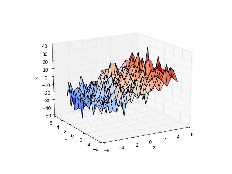
Consider a linear model explaining a variable z (the dependent variable) with 2 variables x andy:

Such a model can be seen in 3D as fitting a plane to a cloud of (x, y, z) points.

 

 

Example: the iris data

Sepal and petal size tend to be related: bigger flowers are bigger! But is there in addition a systematic effect of species?

>>>

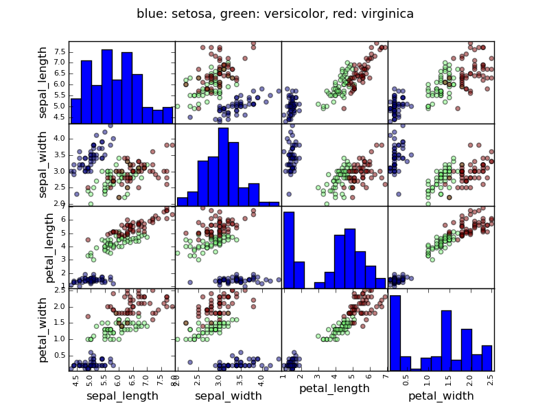
>>> data = pandas.read_csv('examples/iris.csv')

 

>>> model = ols('sepal_width ~ name + petal_length', data).fit()

 

>>> print(model.summary())

 

                            OLS Regression Results

 

==============================================================================

 

Dep. Variable:            sepal_width   R-squared:                       0.478

 

Model:                            OLS   Adj. R-squared:                  0.468

 

Method:                 Least Squares   F-statistic:                     44.63

 

Date:                ...                Prob (F-statistic):           1.58e-20

 

Time:                        ...        Log-Likelihood:                -38.185

 

No. Observations:                 150   AIC:                             84.37

 

Df Residuals:                     146   BIC:                             96.41

 

Df Model:                           3

 

===========================================================================...

 

                         coef    std err          t     P>|t|  [95.0% Conf. Int.]

 

---------------------------------------------------------------------------...

 

Intercept              2.9813      0.099     29.989     0.000      2.785     3.178

 

name[T.versicolor]    -1.4821      0.181     -8.190     0.000     -1.840    -1.124

 

name[T.virginica]     -1.6635      0.256     -6.502     0.000     -2.169    -1.158

 

petal_length           0.2983      0.061      4.920     0.000      0.178     0.418

 

==============================================================================

 

Omnibus:                        2.868   Durbin-Watson:                   1.753

 

Prob(Omnibus):                  0.238   Jarque-Bera (JB):                2.885

 

Skew:                          -0.082   Prob(JB):                        0.236

 

Kurtosis:                       3.659   Cond. No.                         54.0

 

==============================================================================

 

 

3.3   Post-hoc hypothesis testing: analysis of variance (ANOVA)

In the above iris example, we wish to test if the petal length is different between versicolor and virginica, after removing the effect of sepal width. This can be formulated as testing the difference between the coefficient associated to versicolor and virginica in the linear model estimated above (it is an Analysis of Variance, ANOVA). For this, we write a vector of ‘contrast’ on the parameters estimated: we want to test “name[T.versicolor] - name[T.virginica]”, with an ‘F-test’:

>>>

>>> print(model.f_test([0, 1, -1, 0]))

 

<F test: F=array([[ 3.24533535]]), p=[[ 0.07369059]], df_denom=146, df_num=1>

 

Is this difference significant?

 

---

 

Exercice

Going back to the brain size + IQ data, test if the VIQ of male and female are different after removing the effect of brain size, height and weight.

 

4   More visualization: seaborn for statistical exploration

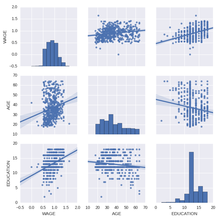
Seaborn combines simple statistical fits with plotting on pandas dataframes.

Let us consider a data giving wages and many other personal information on 500 individuals (Berndt, ER. The Practice of Econometrics. 1991. NY: Addison-Wesley).

>>>

>>> print data

 

     EDUCATION  SOUTH  SEX  EXPERIENCE  UNION      WAGE  AGE  RACE  \

 

0            8      0    1          21      0  0.707570   35     2

 

1            9      0    1          42      0  0.694605   57     3

 

2           12      0    0           1      0  0.824126   19     3

 

3           12      0    0           4      0  0.602060   22     3

 

...

 

We can easily have an intuition on the interactions between continuous variables using seaborn.pairplot to display a scatter matrix:

>>>

>>> import seaborn

 

>>> seaborn.pairplot(data, vars=['WAGE', 'AGE', 'EDUCATION'],

 

...                  kind='reg')

 

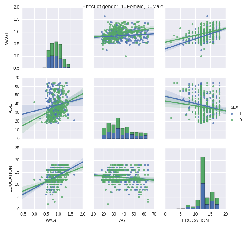
Categorical variables can be plotted as the hue:

>>>

>>> seaborn.pairplot(data, vars=['WAGE', 'AGE', 'EDUCATION'],

 

...                  kind='reg', hue='SEX')

 

5   Testing for interactions

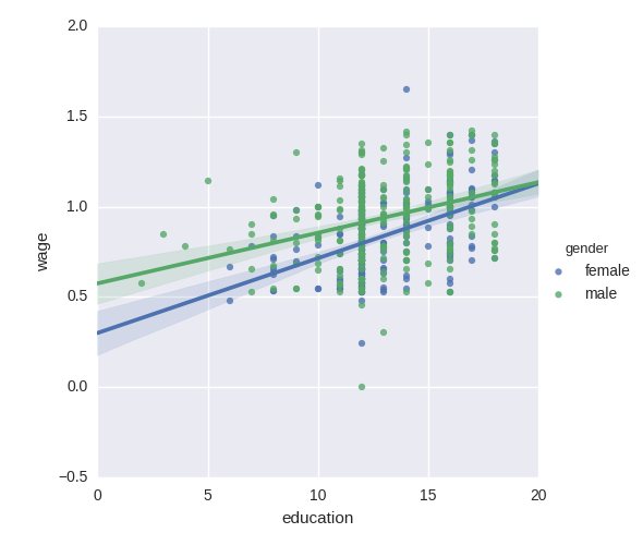
Do wages increase more with education for males than females?

The plot above is made of two different fits. We need to formulate a single model that tests for a variance of slope across the to population. This is done via an“interaction”.

>>>

>>> result = sm.ols(formula='wage ~ education + gender + education * gender',

 

...                 data=data).fit()

 

>>> print(result.summary())

 

...

 

                            coef    std err    t     P>|t|  [95.0% Conf. Int.]

 

------------------------------------------------------------------------------

 

Intercept                   0.2998   0.072    4.173   0.000     0.159   0.441

 

gender[T.male]              0.2750   0.093    2.972   0.003     0.093   0.457

 

education                   0.0415   0.005    7.647   0.000     0.031   0.052

 

education:gender[T.male]   -0.0134   0.007   -1.919   0.056    -0.027   0.000

 

==============================================================================

 

...

 

Can we conclude that education benefits males more than females?

 

Take home messages

• Hypothesis testing and p-value give you the significance of an effect / difference
• Formulas (with categorical variables) enable you to express rich links in your data
• Visualizing your data and simple model fits matters!
• Conditionning (adding factors that can explain all or part of the variation) is important modeling aspect that changes the interpretation.

 

6   Full examples

• Examples
  • Code examples
  • Solutions to the exercises of the course