『TensorFlow』单&双隐藏层自编码器设计

计算图设计

很简单的实践，

• 多了个隐藏层
• 没有上节的高斯噪声
• 网络写法由上节的面向对象改为了函数式编程，

其他没有特别需要注意的，实现如下：

import numpy as np
import matplotlib.pyplot as plt
import tensorflow as tf
from tensorflow.examples.tutorials.mnist import input_data
import os
 
os.environ['TF_CPP_MIN_LOG_LEVEL'] = '2'
 
learning_rate = 0.01                          # 学习率
training_epochs = 20                          # 训练轮数，1轮等于n_samples/batch_size
batch_size = 128                              # batch容量
display_step = 1                              # 展示间隔
example_to_show = 10                          # 展示图像数目
 
n_hidden_units = 256
n_input_units = 784
n_output_units = n_input_units
 
def WeightsVariable(n_in, n_out, name_str):
    return tf.Variable(tf.random_normal([n_in, n_out]), dtype=tf.float32, name=name_str)
 
def biasesVariable(n_out, name_str):
    return tf.Variable(tf.random_normal([n_out]), dtype=tf.float32, name=name_str)
 
def encoder(x_origin, activate_func=tf.nn.sigmoid):
    with tf.name_scope('Layer'):
        Weights = WeightsVariable(n_input_units, n_hidden_units, 'Weights')
        biases = biasesVariable(n_hidden_units, 'biases')
        x_code = activate_func(tf.add(tf.matmul(x_origin, Weights), biases))
    return x_code
 
def decode(x_code, activate_func=tf.nn.sigmoid):
    with tf.name_scope('Layer'):
        Weights = WeightsVariable(n_hidden_units, n_output_units, 'Weights')
        biases = biasesVariable(n_output_units, 'biases')
        x_decode = activate_func(tf.add(tf.matmul(x_code, Weights), biases))
    return x_decode
 
with tf.Graph().as_default():
    with tf.name_scope('Input'):
        X_input = tf.placeholder(tf.float32, [None, n_input_units])
    with tf.name_scope('Encode'):
        X_code = encoder(X_input)
    with tf.name_scope('decode'):
        X_decode = decode(X_code)
    with tf.name_scope('loss'):
        loss = tf.reduce_mean(tf.pow(X_input - X_decode, 2))
    with tf.name_scope('train'):
        Optimizer = tf.train.RMSPropOptimizer(learning_rate)
        train = Optimizer.minimize(loss)
 
    init = tf.global_variables_initializer()
 
    # 因为使用了tf.Graph.as_default()上下文环境
    # 所以下面的记录必须放在上下文里面，否则记录下来的图是空的（get不到上面的default）
    writer = tf.summary.FileWriter(logdir='logs', graph=tf.get_default_graph())
    writer.flush()

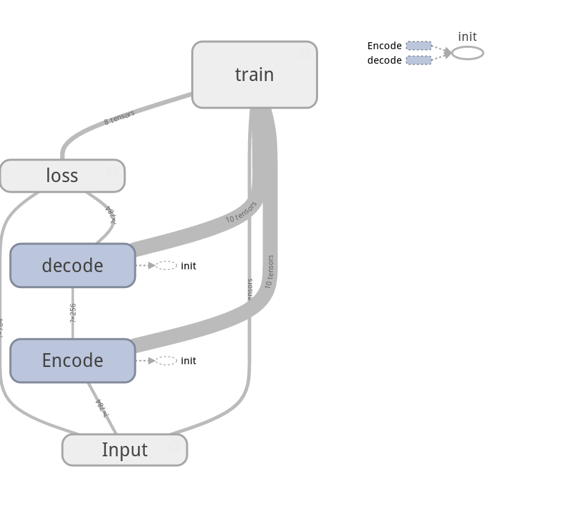
计算图：

训练程序

import numpy as np
import matplotlib.pyplot as plt
import tensorflow as tf
from tensorflow.examples.tutorials.mnist import input_data
import os
 
os.environ['TF_CPP_MIN_LOG_LEVEL'] = '2'
 
learning_rate = 0.01  # 学习率
training_epochs = 20  # 训练轮数，1轮等于n_samples/batch_size
batch_size = 128  # batch容量
display_step = 1  # 展示间隔
example_to_show = 10  # 展示图像数目
 
n_hidden_units = 256
n_input_units = 784
n_output_units = n_input_units
 
def WeightsVariable(n_in, n_out, name_str):
    return tf.Variable(tf.random_normal([n_in, n_out]), dtype=tf.float32, name=name_str)
 
def biasesVariable(n_out, name_str):
    return tf.Variable(tf.random_normal([n_out]), dtype=tf.float32, name=name_str)
 
def encoder(x_origin, activate_func=tf.nn.sigmoid):
    with tf.name_scope('Layer'):
        Weights = WeightsVariable(n_input_units, n_hidden_units, 'Weights')
        biases = biasesVariable(n_hidden_units, 'biases')
        x_code = activate_func(tf.add(tf.matmul(x_origin, Weights), biases))
    return x_code
 
def decode(x_code, activate_func=tf.nn.sigmoid):
    with tf.name_scope('Layer'):
        Weights = WeightsVariable(n_hidden_units, n_output_units, 'Weights')
        biases = biasesVariable(n_output_units, 'biases')
        x_decode = activate_func(tf.add(tf.matmul(x_code, Weights), biases))
    return x_decode
 
with tf.Graph().as_default():
    with tf.name_scope('Input'):
        X_input = tf.placeholder(tf.float32, [None, n_input_units])
    with tf.name_scope('Encode'):
        X_code = encoder(X_input)
    with tf.name_scope('decode'):
        X_decode = decode(X_code)
    with tf.name_scope('loss'):
        loss = tf.reduce_mean(tf.pow(X_input - X_decode, 2))
    with tf.name_scope('train'):
        Optimizer = tf.train.RMSPropOptimizer(learning_rate)
        train = Optimizer.minimize(loss)
 
    init = tf.global_variables_initializer()
 
    # 因为使用了tf.Graph.as_default()上下文环境
    # 所以下面的记录必须放在上下文里面，否则记录下来的图是空的（get不到上面的default）
    writer = tf.summary.FileWriter(logdir='logs', graph=tf.get_default_graph())
    writer.flush()
 
    mnist = input_data.read_data_sets('../Mnist_data/', one_hot=True)
 
    with tf.Session() as sess:
        sess.run(init)
        total_batch = int(mnist.train.num_examples / batch_size)
        for epoch in range(training_epochs):
            for i in range(total_batch):
                batch_xs, batch_ys = mnist.train.next_batch(batch_size)
                _, Loss = sess.run([train, loss], feed_dict={X_input: batch_xs})
                Loss = sess.run(loss, feed_dict={X_input: batch_xs})
            if epoch % display_step == 0:
                print('Epoch: %04d' % (epoch + 1), 'loss= ', '{:.9f}'.format(Loss))
        writer.close()
        print('训练完毕！')
 
        '''比较输入和输出的图像'''
        # 输出图像获取
        reconstructions = sess.run(X_decode, feed_dict={X_input: mnist.test.images[:example_to_show]})
        # 画布建立
        f, a = plt.subplots(2, 10, figsize=(10, 2))
        for i in range(example_to_show):
            a[0][i].imshow(np.reshape(mnist.test.images[i], (28, 28)))
            a[1][i].imshow(np.reshape(reconstructions[i], (28, 28)))
        f.show()  # 渲染图像
        plt.draw()  # 刷新图像
        # plt.waitforbuttonpress()

debug一上午的收获：接受sess.run输出的变量名不要和tensor节点的变量名重复，会出错的... ...好低级的错误。mmdz

比较图像一部分之前没做过，介绍了matplotlib.pyplot的花式用法，

　　原来plt.subplots()是会返回 画布句柄 & 子图集合 句柄的，子图集合句柄可以像数组一样调用子图

　　 pyplot是有show()和draw()两个方法的，show是展示出画布，draw会刷新原图，可以交互的修改画布

　　 waitforbuttonpress()监听键盘按键如果用户按的是键盘,返回True,如果是其他(如鼠标单击),则返回False

另，发现用surface写程序其实还挺带感... ...

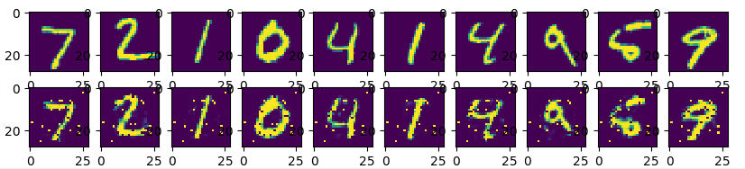
输出图像如下：

双隐藏层版本

import numpy as np
import matplotlib.pyplot as plt
import tensorflow as tf
from tensorflow.examples.tutorials.mnist import input_data
import os
 
os.environ['TF_CPP_MIN_LOG_LEVEL'] = '2'
 
batch_size = 128  # batch容量
display_step = 1  # 展示间隔
learning_rate = 0.01  # 学习率
training_epochs = 20  # 训练轮数，1轮等于n_samples/batch_size
example_to_show = 10  # 展示图像数目
 
n_hidden1_units = 256  # 第一隐藏层
n_hidden2_units = 128  # 第二隐藏层
n_input_units = 784
n_output_units = n_input_units
 
def WeightsVariable(n_in, n_out, name_str):
    return tf.Variable(tf.random_normal([n_in, n_out]), dtype=tf.float32, name=name_str)
 
def biasesVariable(n_out, name_str):
    return tf.Variable(tf.random_normal([n_out]), dtype=tf.float32, name=name_str)
 
def encoder(x_origin, activate_func=tf.nn.sigmoid):
    with tf.name_scope('Layer1'):
        Weights = WeightsVariable(n_input_units, n_hidden1_units, 'Weights')
        biases = biasesVariable(n_hidden1_units, 'biases')
        x_code1 = activate_func(tf.add(tf.matmul(x_origin, Weights), biases))
    with tf.name_scope('Layer2'):
        Weights = WeightsVariable(n_hidden1_units, n_hidden2_units, 'Weights')
        biases = biasesVariable(n_hidden2_units, 'biases')
        x_code2 = activate_func(tf.add(tf.matmul(x_code1, Weights), biases))
    return x_code2
 
def decode(x_code, activate_func=tf.nn.sigmoid):
    with tf.name_scope('Layer1'):
        Weights = WeightsVariable(n_hidden2_units, n_hidden1_units, 'Weights')
        biases = biasesVariable(n_hidden1_units, 'biases')
        x_decode1 = activate_func(tf.add(tf.matmul(x_code, Weights), biases))
    with tf.name_scope('Layer2'):
        Weights = WeightsVariable(n_hidden1_units, n_output_units, 'Weights')
        biases = biasesVariable(n_output_units, 'biases')
        x_decode2 = activate_func(tf.add(tf.matmul(x_decode1, Weights), biases))
    return x_decode2
 
with tf.Graph().as_default():
    with tf.name_scope('Input'):
        X_input = tf.placeholder(tf.float32, [None, n_input_units])
    with tf.name_scope('Encode'):
        X_code = encoder(X_input)
    with tf.name_scope('decode'):
        X_decode = decode(X_code)
    with tf.name_scope('loss'):
        loss = tf.reduce_mean(tf.pow(X_input - X_decode, 2))
    with tf.name_scope('train'):
        Optimizer = tf.train.RMSPropOptimizer(learning_rate)
        train = Optimizer.minimize(loss)
 
    init = tf.global_variables_initializer()
 
    # 因为使用了tf.Graph.as_default()上下文环境
    # 所以下面的记录必须放在上下文里面，否则记录下来的图是空的（get不到上面的default）
    writer = tf.summary.FileWriter(logdir='logs', graph=tf.get_default_graph())
    writer.flush()
 
    mnist = input_data.read_data_sets('../Mnist_data/', one_hot=True)
 
    with tf.Session() as sess:
        sess.run(init)
        total_batch = int(mnist.train.num_examples / batch_size)
        for epoch in range(training_epochs):
            for i in range(total_batch):
                batch_xs, batch_ys = mnist.train.next_batch(batch_size)
                _, Loss = sess.run([train, loss], feed_dict={X_input: batch_xs})
                Loss = sess.run(loss, feed_dict={X_input: batch_xs})
            if epoch % display_step == 0:
                print('Epoch: %04d' % (epoch + 1), 'loss= ', '{:.9f}'.format(Loss))
        writer.close()
        print('训练完毕！')
 
        '''比较输入和输出的图像'''
        # 输出图像获取
        reconstructions = sess.run(X_decode, feed_dict={X_input: mnist.test.images[:example_to_show]})
        # 画布建立
        f, a = plt.subplots(2, 10, figsize=(10, 2))
        for i in range(example_to_show):
            a[0][i].imshow(np.reshape(mnist.test.images[i], (28, 28)))
            a[1][i].imshow(np.reshape(reconstructions[i], (28, 28)))
        f.show()  # 渲染图像
        plt.draw()  # 刷新图像
        # plt.waitforbuttonpress()

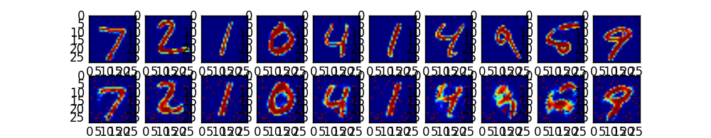
输出图像如下：

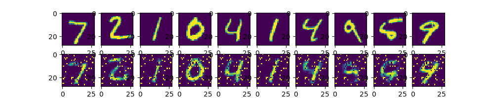
由于压缩到128个节点损失信息过多，所以结果不如之前单层的好。

有意思的是我们把256的那层改成128（也就是双128）后，结果反而比上面的要好：

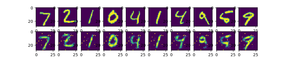
但是仍然比不上单隐藏层，数据比较简单时候复杂网络效果可能不那么好（loss值我没有截取，但实际上是这样，虽然不同网络loss直接比较没什么意义），当然，也有可能是复杂网络没收敛的结果。

可视化双隐藏层自编码器

import tensorflow as tf
from tensorflow.examples.tutorials.mnist import input_data
import os
 
os.environ['TF_CPP_MIN_LOG_LEVEL'] = '2'
 
batch_size = 128  # batch容量
display_step = 1  # 展示间隔
learning_rate = 0.01  # 学习率
training_epochs = 20  # 训练轮数，1轮等于n_samples/batch_size
example_to_show = 10  # 展示图像数目
 
n_hidden1_units = 256  # 第一隐藏层
n_hidden2_units = 128  # 第二隐藏层
n_input_units = 784
n_output_units = n_input_units
 
def variable_summaries(var): #<---
    """
    可视化变量全部相关参数
    :param var:
    :return:
    """
    with tf.name_scope('summaries'):
        mean = tf.reduce_mean(var)
        tf.summary.histogram('mean', mean)
        with tf.name_scope('stddev'):
            stddev = tf.sqrt(tf.reduce_mean(tf.square(var - mean)))
            tf.summary.scalar('stddev', stddev)  # 注意，这是标量
            tf.summary.scalar('max', tf.reduce_max(var))
            tf.summary.scalar('min', tf.reduce_min(var))
            tf.summary.histogram('histogram', var)
 
def WeightsVariable(n_in,n_out,name_str):
    return tf.Variable(tf.random_normal([n_in,n_out]),dtype=tf.float32,name=name_str)
 
def biasesVariable(n_out,name_str):
    return tf.Variable(tf.random_normal([n_out]),dtype=tf.float32,name=name_str)
 
def encoder(x_origin,activate_func=tf.nn.sigmoid):
    with tf.name_scope('Layer1'):
        Weights = WeightsVariable(n_input_units,n_hidden1_units,'Weights')
        biases = biasesVariable(n_hidden1_units,'biases')
        x_code1 = activate_func(tf.add(tf.matmul(x_origin,Weights),biases))
        variable_summaries(Weights) #<---
        variable_summaries(biases) #<---
    with tf.name_scope('Layer2'):
        Weights = WeightsVariable(n_hidden1_units,n_hidden2_units,'Weights')
        biases = biasesVariable(n_hidden2_units,'biases')
        x_code2 = activate_func(tf.add(tf.matmul(x_code1,Weights),biases))
        variable_summaries(Weights) #<---
        variable_summaries(biases) #<---
    return x_code2
 
def decode(x_code,activate_func=tf.nn.sigmoid):
    with tf.name_scope('Layer1'):
        Weights = WeightsVariable(n_hidden2_units,n_hidden1_units,'Weights')
        biases = biasesVariable(n_hidden1_units,'biases')
        x_decode1 = activate_func(tf.add(tf.matmul(x_code,Weights),biases))
        variable_summaries(Weights) #<---
        variable_summaries(biases) #<---
    with tf.name_scope('Layer2'):
        Weights = WeightsVariable(n_hidden1_units,n_output_units,'Weights')
        biases = biasesVariable(n_output_units,'biases')
        x_decode2 = activate_func(tf.add(tf.matmul(x_decode1,Weights),biases))
        variable_summaries(Weights) #<---
        variable_summaries(biases) #<---
    return x_decode2
 
with tf.Graph().as_default():
    with tf.name_scope('Input'):
        X_input = tf.placeholder(tf.float32,[None,n_input_units])
    with tf.name_scope('Encode'):
        X_code = encoder(X_input)
    with tf.name_scope('decode'):
        X_decode = decode(X_code)
    with tf.name_scope('loss'):
        loss = tf.reduce_mean(tf.pow(X_input - X_decode,2))
    with tf.name_scope('train'):
        Optimizer = tf.train.RMSPropOptimizer(learning_rate)
        train = Optimizer.minimize(loss)
 
    # 标量汇总
    with tf.name_scope('LossSummary'):
        tf.summary.scalar('loss',loss)
        tf.summary.scalar('learning_rate',learning_rate)
 
    # 图像展示
    with tf.name_scope('ImageSummary'):
        image_original = tf.reshape(X_input,[-1, 28, 28, 1])
        image_reconstruction = tf.reshape(X_decode, [-1, 28, 28, 1])
        tf.summary.image('image_original', image_original, 9)
        tf.summary.image('image_recinstruction', image_reconstruction, 9)
 
    # 汇总
    merged_summary = tf.summary.merge_all()
 
    init = tf.global_variables_initializer()
 
    writer = tf.summary.FileWriter(logdir='logs', graph=tf.get_default_graph())
    writer.flush()
 
    mnist = input_data.read_data_sets('../Mnist_data/', one_hot=True)
 
    with tf.Session() as sess:
        sess.run(init)
        total_batch = int(mnist.train.num_examples / batch_size)
        for epoch in range(training_epochs):
            for i in range(total_batch):
                batch_xs,batch_ys = mnist.train.next_batch(batch_size)
                _,Loss = sess.run([train,loss],feed_dict={X_input: batch_xs})
                Loss = sess.run(loss,feed_dict={X_input: batch_xs})
            if epoch % display_step == 0:
                print('Epoch: %04d' % (epoch + 1),'loss= ','{:.9f}'.format(Loss))
                summary_str = sess.run(merged_summary,feed_dict={X_input: batch_xs}) #<---
                writer.add_summary(summary_str,epoch) #<---
                writer.flush() #<---
        writer.close()
        print('训练完毕！')

几个有意思的发现，

　　使用之前的图像输出方式时，win下matplotlib.pyplot的绘画框会立即退出，所以要使用 plt.waitforbuttonpress() 命令。

　　win下使用plt绘画色彩和linux不一样，效果如下：

　　

输出图如下：

对比图像如下（截自tensorboard）：