<转>机器学习笔记之奇异值分解的几何解释与简单应用

看到的一篇比较好的关于SVD几何解释与简单应用的文章，其实是有中文译本的，但是翻译的太烂，还不如直接看英文原文的。课本上学的往往是知其然不知其所以然，希望这篇文能为所有初学svd的童鞋提供些直观的认识吧。

A sigular value decomposition

目录(?)[-]

1. Introduction
2. The geometry of linear transformations
3. The singular value decomposition
4. How do we find the singular decomposition
5. Another example
6. Data compression
7. Noise reduction
8. Data analysis
9. Summary
10. References

 

Introduction

The topic of this article, the singular value decomposition, is one that should be a part of the standard mathematics undergraduate curriculum but all too often slips between the cracks. Besides being rather intuitive, these decompositions are incredibly useful. For instance, Netflix, the online movie rental company, is currently offering a $1 million prize for anyone who can improve the accuracy of its movie recommendation system by 10%. Surprisingly, this seemingly modest problem turns out to be quite challenging, and the groups involved are now using rather sophisticated techniques. At the heart of all of them is the singular value decomposition.

A singular value decomposition provides a convenient way for breaking a matrix, which perhaps contains some data we are interested in, into simpler, meaningful pieces. In this article, we will offer a geometric explanation of singular value decompositions and look at some of the applications of them.

The geometry of linear transformations

Let us begin by looking at some simple matrices, namely those with two rows and two columns. Our first example is the diagonal matrix

Geometrically, we may think of a matrix like this as taking a point (x, y) in the plane and transforming it into another point using matrix multiplication:

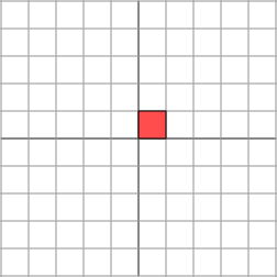
The effect of this transformation is shown below: the plane is horizontally stretched by a factor of 3, while there is no vertical change.

Now let's look at

which produces this effect

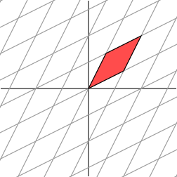It is not so clear how to describe simply the geometric effect of the transformation. However, let's rotate our grid through a 45 degree angle and see what happens.

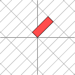Ah ha. We see now that this new grid is transformed in the same way that the original grid was transformed by the diagonal matrix: the grid is stretched by a factor of 3 in one direction.

This is a very special situation that results from the fact that the matrix M is symmetric; that is, the transpose of M, the matrix obtained by flipping the entries about the diagonal, is equal to M. If we have a symmetric 2  2 matrix, it turns out that we may always rotate the grid in the domain so that the matrix acts by stretching and perhaps reflecting in the two directions. In other words, symmetric matrices behave like diagonal matrices.

Said with more mathematical precision, given a symmetric matrix M, we may find a set of orthogonal vectors v_i so that Mv_i is a scalar multiple of v_i; that is

Mv_i = λ_iv_i

where λ_i is a scalar. Geometrically, this means that the vectors v_i are simply stretched and/or reflected when multiplied by M. Because of this property, we call the vectors v_i eigenvectors of M; the scalars λ_i are called eigenvalues. An important fact, which is easily verified, is that eigenvectors of a symmetric matrix corresponding to different eigenvalues are orthogonal.

If we use the eigenvectors of a symmetric matrix to align the grid, the matrix stretches and reflects the grid in the same way that it does the eigenvectors.

The geometric description we gave for this linear transformation is a simple one: the grid is simply stretched in one direction. For more general matrices, we will ask if we can find an orthogonal grid that is transformed into another orthogonal grid. Let's consider a final example using a matrix that is not symmetric:

This matrix produces the geometric effect known as a shear.

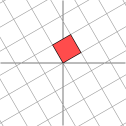
It's easy to find one family of eigenvectors along the horizontal axis. However, our figure above shows that these eigenvectors cannot be used to create an orthogonal grid that is transformed into another orthogonal grid. Nonetheless, let's see what happens when we rotate the grid first by 30 degrees,

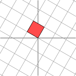
Notice that the angle at the origin formed by the red parallelogram on the right has increased. Let's next rotate the grid by 60 degrees.

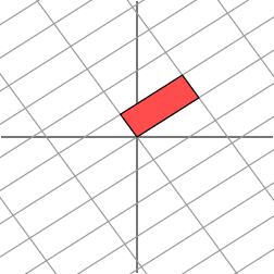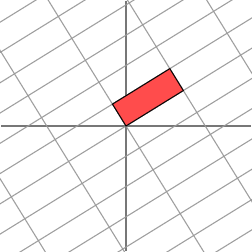
Hmm. It appears that the grid on the right is now almost orthogonal. In fact, by rotating the grid in the domain by an angle of roughly 58.28 degrees, both grids are now orthogonal.

The singular value decomposition

This is the geometric essence of the singular value decomposition for 2  2 matrices: for any 2  2 matrix, we may find an orthogonal grid that is transformed into another orthogonal grid.

We will express this fact using vectors: with an appropriate choice of orthogonal unit vectors v₁ and v₂, the vectors Mv₁ andMv₂ are orthogonal.

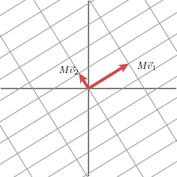We will use u₁ and u₂ to denote unit vectors in the direction of Mv₁ and Mv₂. The lengths of Mv₁ and Mv₂--denoted by σ₁ and σ₂--describe the amount that the grid is stretched in those particular directions. These numbers are called the singular valuesof M. (In this case, the singular values are the golden ratio and its reciprocal, but that is not so important here.)

We therefore have

Mv₁ = σ₁u₁ 
Mv₂ = σ₂u₂

We may now give a simple description for how the matrix M treats a general vector x. Since the vectors v₁ and v₂ are orthogonal unit vectors, we have

x = (v₁x) v₁ + (v₂x) v₂

This means that

Mx = (v₁x) Mv₁ + (v₂x) Mv₂ 
Mx = (v₁x) σ₁u₁ + (v₂x) σ₂u₂

Remember that the dot product may be computed using the vector transpose

vx = v^Tx

which leads to

Mx = u₁σ₁ v₁^Tx + u₂σ₂ v₂^Tx 
M = u₁σ₁ v₁^T + u₂σ₂ v₂^T

This is usually expressed by writing

M = UΣV^T

where U is a matrix whose columns are the vectors u₁ and u₂, Σ is a diagonal matrix whose entries are σ₁ and σ₂, and V is a matrix whose columns are v₁ and v₂. The superscript T on the matrix V denotes the matrix transpose of V.

This shows how to decompose the matrix M into the product of three matrices: V describes an orthonormal basis in the domain, and U describes an orthonormal basis in the co-domain, and Σ describes how much the vectors in V are stretched to give the vectors in U.

How do we find the singular decomposition?

The power of the singular value decomposition lies in the fact that we may find it for any matrix. How do we do it? Let's look at our earlier example and add the unit circle in the domain. Its image will be an ellipse whose major and minor axes define the orthogonal grid in the co-domain.

Notice that the major and minor axes are defined by Mv₁ and Mv₂. These vectors therefore are the longest and shortest vectors among all the images of vectors on the unit circle.

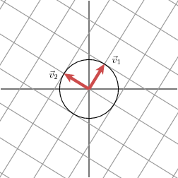In other words, the function |Mx| on the unit circle has a maximum at v₁ and a minimum at v₂. This reduces the problem to a rather standard calculus problem in which we wish to optimize a function over the unit circle. It turns out that the critical points of this function occur at the eigenvectors of the matrix M^TM. Since this matrix is symmetric, eigenvectors corresponding to different eigenvalues will be orthogonal. This gives the family of vectors v_i.

The singular values are then given by σ_i = |Mv_i|, and the vectors u_i are obtained as unit vectors in the direction of Mv_i. But why are the vectors u_i orthogonal?

To explain this, we will assume that σ_i and σ_j are distinct singular values. We have

Mv_i = σ_iu_i 
Mv_j = σ_ju_j.

Let's begin by looking at the expression Mv_iMv_j and assuming, for convenience, that the singular values are non-zero. On one hand, this expression is zero since the vectors v_i, which are eigenvectors of the symmetric matrix M^TM are orthogonal to one another:

Mv_i Mv_j = v_i^TM^T Mv_j = v_i M^TMv_j = λ_jv_i v_j = 0.

On the other hand, we have

Mv_i Mv_j = σ_iσ_j u_i u_j = 0

Therefore, u_i and u_j are othogonal so we have found an orthogonal set of vectors v_i that is transformed into another orthogonal set u_i. The singular values describe the amount of stretching in the different directions.

In practice, this is not the procedure used to find the singular value decomposition of a matrix since it is not particularly efficient or well-behaved numerically.

Another example

Let's now look at the singular matrix

The geometric effect of this matrix is the following:

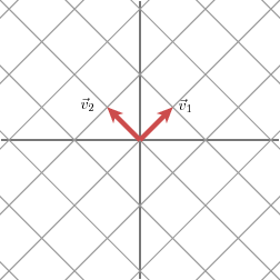In this case, the second singular value is zero so that we may write:

M = u₁σ₁ v₁^T.

In other words, if some of the singular values are zero, the corresponding terms do not appear in the decomposition for M. In this way, we see that the rank of M, which is the dimension of the image of the linear transformation, is equal to the number of non-zero singular values.

Data compression

Singular value decompositions can be used to represent data efficiently. Suppose, for instance, that we wish to transmit the following image, which consists of an array of 15  25 black or white pixels.

Since there are only three types of columns in this image, as shown below, it should be possible to represent the data in a more compact form.

  

We will represent the image as a 15  25 matrix in which each entry is either a 0, representing a black pixel, or 1, representing white. As such, there are 375 entries in the matrix.

If we perform a singular value decomposition on M, we find there are only three non-zero singular values.

σ₁ = 14.72 
σ₂ = 5.22 
σ₃ = 3.31

Therefore, the matrix may be represented as

M=u₁σ₁ v₁^T + u₂σ₂ v₂^T + u₃σ₃ v₃^T

This means that we have three vectors v_i, each of which has 15 entries, three vectors u_i, each of which has 25 entries, and three singular values σ_i. This implies that we may represent the matrix using only 123 numbers rather than the 375 that appear in the matrix. In this way, the singular value decomposition discovers the redundancy in the matrix and provides a format for eliminating it.

Why are there only three non-zero singular values? Remember that the number of non-zero singular values equals the rank of the matrix. In this case, we see that there are three linearly independent columns in the matrix, which means that the rank will be three.

Noise reduction

The previous example showed how we can exploit a situation where many singular values are zero. Typically speaking, the large singular values point to where the interesting information is. For example, imagine we have used a scanner to enter this image into our computer. However, our scanner introduces some imperfections (usually called "noise") in the image.

We may proceed in the same way: represent the data using a 15  25 matrix and perform a singular value decomposition. We find the following singular values:

σ₁ = 14.15 
σ₂ = 4.67 
σ₃ = 3.00 
σ₄ = 0.21 
σ₅ = 0.19 
... 
σ₁₅ = 0.05

Clearly, the first three singular values are the most important so we will assume that the others are due to the noise in the image and make the approximation

M  u₁σ₁ v₁^T + u₂σ₂ v₂^T + u₃σ₃ v₃^T

This leads to the following improved image.

Noisy image	Improved image

Data analysis

Noise also arises anytime we collect data: no matter how good the instruments are, measurements will always have some error in them. If we remember the theme that large singular values point to important features in a matrix, it seems natural to use a singular value decomposition to study data once it is collected.

As an example, suppose that we collect some data as shown below:

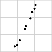
We may take the data and put it into a matrix:

-1.03	0.74	-0.02	0.51	-1.31	0.99	0.69	-0.12	-0.72	1.11
-2.23	1.61	-0.02	0.88	-2.39	2.02	1.62	-0.35	-1.67	2.46

and perform a singular value decomposition. We find the singular values

σ₁ = 6.04 
σ₂ = 0.22

With one singular value so much larger than the other, it may be safe to assume that the small value of σ₂ is due to noise in the data and that this singular value would ideally be zero. In that case, the matrix would have rank one meaning that all the data lies on the line defined by u_i.

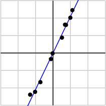
This brief example points to the beginnings of a field known as principal component analysis, a set of techniques that uses singular values to detect dependencies and redundancies in data.

In a similar way, singular value decompositions can be used to detect groupings in data, which explains why singular value decompositions are being used in attempts to improve Netflix's movie recommendation system. Ratings of movies you have watched allow a program to sort you into a group of others whose ratings are similar to yours. Recommendations may be made by choosing movies that others in your group have rated highly.

Summary

As mentioned at the beginning of this article, the singular value decomposition should be a central part of an undergraduate mathematics major's linear algebra curriculum. Besides having a rather simple geometric explanation, the singular value decomposition offers extremely effective techniques for putting linear algebraic ideas into practice. All too often, however, a proper treatment in an undergraduate linear algebra course seems to be missing.

This article has been somewhat impressionistic: I have aimed to provide some intuitive insights into the central idea behind singular value decompositions and then illustrate how this idea can be put to good use. More rigorous accounts may be readily found.

References:

• Gilbert Strang, Linear Algebra and Its Applications. Brooks Cole.

  Strang's book is something of a classic though some may find it to be a little too formal.

• William H. Press et al, Numercial Recipes in C: The Art of Scientific Computing. Cambridge University Press. 

  Authoritative, yet highly readable. Older versions are available online.

• Dan Kalman, A Singularly Valuable Decomposition: The SVD of a Matrix, The College Mathematics Journal 27 (1996), 2-23. 

  Kalman's article, like this one, aims to improve the profile of the singular value decomposition. It also a description of how least-squares computations are facilitated by the decomposition.

• If You Liked This, You're Sure to Love That, The New York Times, November 21, 2008. 

  This article describes Netflix's prize competition as well as some of the challenges associated with it.

David Austin
Grand Valley State University 
david at merganser.math.gvsu.edu

Those who can access JSTOR can find at least of the papers mentioned above there. For those with access, the American Mathematical Society's MathSciNet can be used to get additional bibliographic information and reviews of some these materials. Some of the items above can be accessed via the ACM Portal , which also provides bibliographic services.