Policy Gradient Algorithms
Policy Gradient Algorithms
2019-10-02 17:37:47
This blog is from: https://lilianweng.github.io/lil-log/2018/04/08/policy-gradient-algorithms.html
Abstract: In this post, we are going to look deep into policy gradient, why it works, and many new policy gradient algorithms proposed in recent years: vanilla policy gradient, actor-critic, off-policy actor-critic, A3C, A2C, DPG, DDPG, D4PG, MADDPG, TRPO, PPO, ACER, ACTKR, SAC, TD3 & SVPG.
What is Policy Gradient
Policy gradient is an approach to solve reinforcement learning problems. If you haven’t looked into the field of reinforcement learning, please first read the section “A (Long) Peek into Reinforcement Learning » Key Concepts” for the problem definition and key concepts.
Notations
Here is a list of notations to help you read through equations in the post easily.
| Symbol | Meaning |
|---|---|
| s∈Ss∈S | States. |
| a∈Aa∈A | Actions. |
| r∈Rr∈R | Rewards. |
| St,At,RtSt,At,Rt | State, action, and reward at time step t of one trajectory. I may occasionally use st,at,rtst,at,rt as well. |
| γγ | Discount factor; penalty to uncertainty of future rewards; 0<γ≤10<γ≤1. |
| GtGt | Return; or discounted future reward; Gt=∑∞k=0γkRt+k+1Gt=∑k=0∞γkRt+k+1. |
| P(s′,r|s,a)P(s′,r|s,a) | Transition probability of getting to the next state s’ from the current state s with action a and reward r. |
| π(a|s)π(a|s) | Stochastic policy (agent behavior strategy); πθ(.)πθ(.) is a policy parameterized by θ. |
| μ(s)μ(s) | Deterministic policy; we can also label this as π(s)π(s), but using a different letter gives better distinction so that we can easily tell when the policy is stochastic or deterministic without further explanation. Either ππ or μμ is what a reinforcement learning algorithm aims to learn. |
| V(s)V(s) | State-value function measures the expected return of state s; Vw(.)Vw(.) is a value function parameterized by w. |
| Vπ(s)Vπ(s) | The value of state s when we follow a policy π; Vπ(s)=Ea∼π[Gt|St=s]Vπ(s)=Ea∼π[Gt|St=s]. |
| Q(s,a)Q(s,a) | Action-value function is similar to V(s)V(s), but it assesses the expected return of a pair of state and action (s, a); Qw(.)Qw(.) is a action value function parameterized by w. |
| Qπ(s,a)Qπ(s,a) | Similar to Vπ(.)Vπ(.), the value of (state, action) pair when we follow a policy π; Qπ(s,a)=Ea∼π[Gt|St=s,At=a]Qπ(s,a)=Ea∼π[Gt|St=s,At=a]. |
| A(s,a)A(s,a) | Advantage function, A(s,a)=Q(s,a)−V(s)A(s,a)=Q(s,a)−V(s); it can be considered as another version of Q-value with lower variance by taking the state-value off as the baseline. |
Policy Gradient
The goal of reinforcement learning is to find an optimal behavior strategy for the agent to obtain optimal rewards. The policy gradient methods target at modeling and optimizing the policy directly. The policy is usually modeled with a parameterized function respect to θ, πθ(a|s)πθ(a|s). The value of the reward (objective) function depends on this policy and then various algorithms can be applied to optimize θ for the best reward.
The reward function is defined as:
where dπ(s)dπ(s) is the stationary distribution of Markov chain for πθπθ (on-policy state distribution under π). For simplicity, the θ parameter would be omitted for the policy πθπθ when the policy is present in the subscript of other functions; for example, dπdπ and QπQπ should be dπθdπθ and QπθQπθ if written in full. Imagine that you can travel along the Markov chain’s states forever, and eventually, as the time progresses, the probability of you ending up with one state becomes unchanged — this is the stationary probability for πθπθ. dπ(s)=limt→∞P(st=s|s0,πθ)dπ(s)=limt→∞P(st=s|s0,πθ) is the probability that st=sst=s when starting from s0s0 and following policy πθπθ for t steps. Actually, the existence of the stationary distribution of Markov chain is one main reason for why PageRank algorithm works. If you want to read more, check this.
It is natural to expect policy-based methods are more useful in the continuous space. Because there is an infinite number of actions and (or) states to estimate the values for and hence value-based approaches are way too expensive computationally in the continuous space. For example, in generalized policy iteration, the policy improvement step argmaxa∈AQπ(s,a)argmaxa∈AQπ(s,a) requires a full scan of the action space, suffering from the curse of dimensionality.
Using gradient ascent, we can move θ toward the direction suggested by the gradient ∇θJ(θ)∇θJ(θ) to find the best θ for πθπθ that produces the highest return.
Policy Gradient Theorem
Computing the gradient ∇θJ(θ)∇θJ(θ) is tricky because it depends on both the action selection (directly determined by πθπθ) and the stationary distribution of states following the target selection behavior (indirectly determined by πθπθ). Given that the environment is generally unknown, it is difficult to estimate the effect on the state distribution by a policy update.
Luckily, the policy gradient theorem comes to save the world! Woohoo! It provides a nice reformation of the derivative of the objective function to not involve the derivative of the state distribution dπ(.)dπ(.) and simplify the gradient computation ∇θJ(θ)∇θJ(θ) a lot.
Proof of Policy Gradient Theorem
This session is pretty dense, as it is the time for us to go through the proof (Sutton & Barto, 2017; Sec. 13.1) and figure out why the policy gradient theorem is correct.
We first start with the derivative of the state value function:
Now we have:
This equation has a nice recursive form (see the red parts!) and the future state value function Vπ(s′)Vπ(s′) can be repeated unrolled by following the same equation.
Let’s consider the following visitation sequence and label the probability of transitioning from state s to state x with policy πθπθ after k step as ρπ(s→x,k)ρπ(s→x,k).
- When k = 0: ρπ(s→s,k=0)=1ρπ(s→s,k=0)=1.
- When k = 1, we scan through all possible actions and sum up the transition probabilities to the target state: ρπ(s→s′,k=1)=∑aπθ(a|s)P(s′|s,a)ρπ(s→s′,k=1)=∑aπθ(a|s)P(s′|s,a).
- Imagine that the goal is to go from state s to x after k+1 steps while following policy πθπθ. We can first travel from s to a middle point s’ (any state can be a middle point, s′∈Ss′∈S) after k steps and then go to the final state x during the last step. In this way, we are able to update the visitation probability recursively: ρπ(s→x,k+1)=∑s′ρπ(s→s′,k)ρπ(s′→x,1)ρπ(s→x,k+1)=∑s′ρπ(s→s′,k)ρπ(s′→x,1).
Then we go back to unroll the recursive representation of ∇θVπ(s)∇θVπ(s)! Let ϕ(s)=∑a∈A∇θπθ(a|s)Qπ(s,a)ϕ(s)=∑a∈A∇θπθ(a|s)Qπ(s,a) to simplify the maths. If we keep on extending ∇θVπ(.)∇θVπ(.) infinitely, it is easy to find out that we can transition from the starting state s to any state after any number of steps in this unrolling process and by summing up all the visitation probabilities, we get ∇θVπ(s)∇θVπ(s)!
The nice rewriting above allows us to exclude the derivative of Q-value function, ∇θQπ(s,a)∇θQπ(s,a). By plugging it into the objective function J(θ)J(θ), we are getting the following:
In the episodic case, the constant of proportionality (∑sη(s)∑sη(s)) is the average length of an episode; in the continuing case, it is 1 (Sutton & Barto, 2017; Sec. 13.2). The gradient can be further written as:
Where EπEπ refers to Es∼dπ,a∼πθEs∼dπ,a∼πθ when both state and action distributions follow the policy πθπθ (on policy).
The policy gradient theorem lays the theoretical foundation for various policy gradient algorithms. This vanilla policy gradient update has no bias but high variance. Many following algorithms were proposed to reduce the variance while keeping the bias unchanged.
Here is a nice summary of a general form of policy gradient methods borrowed from the GAE (general advantage estimation) paper (Schulman et al., 2016) and this post thoroughly discussed several components in GAE , highly recommended.
Fig. 1. A general form of policy gradient methods. (Image source: Schulman et al., 2016)
Policy Gradient Algorithms
Tons of policy gradient algorithms have been proposed during recent years and there is no way for me to exhaust them. I’m introducing some of them that I happened to know and read about.
REINFORCE
REINFORCE (Monte-Carlo policy gradient) relies on an estimated return by Monte-Carlo methods using episode samples to update the policy parameter θθ. REINFORCE works because the expectation of the sample gradient is equal to the actual gradient:
Therefore we are able to measure GtGt from real sample trajectories and use that to update our policy gradient. It relies on a full trajectory and that’s why it is a Monte-Carlo method.
The process is pretty straightforward:
- Initialize the policy parameter θ at random.
- Generate one trajectory on policy πθπθ: S1,A1,R2,S2,A2,…,STS1,A1,R2,S2,A2,…,ST.
- For t=1, 2, … , T:
- Estimate the the return GtGt;
- Update policy parameters: θ←θ+αγtGt∇θlnπθ(At|St)θ←θ+αγtGt∇θlnπθ(At|St)
A widely used variation of REINFORCE is to subtract a baseline value from the return GtGt to reduce the variance of gradient estimation while keeping the bias unchanged (Remember we always want to do this when possible). For example, a common baseline is to subtract state-value from action-value, and if applied, we would use advantage A(s,a)=Q(s,a)−V(s)A(s,a)=Q(s,a)−V(s) in the gradient ascent update. This post nicely explained why a baseline works for reducing the variance, in addition to a set of fundamentals of policy gradient.
Actor-Critic
Two main components in policy gradient are the policy model and the value function. It makes a lot of sense to learn the value function in addition to the policy, since knowing the value function can assist the policy update, such as by reducing gradient variance in vanilla policy gradients, and that is exactly what the Actor-Critic method does.
Actor-critic methods consist of two models, which may optionally share parameters:
- Critic updates the value function parameters w and depending on the algorithm it could be action-value Qw(a|s)Qw(a|s) or state-value Vw(s)Vw(s).
- Actor updates the policy parameters θ for πθ(a|s)πθ(a|s), in the direction suggested by the critic.
Let’s see how it works in a simple action-value actor-critic algorithm.
- Initialize s, θ, w at random; sample a∼πθ(a|s)a∼πθ(a|s).
- For t=1…Tt=1…T:
- Sample reward rt∼R(s,a)rt∼R(s,a) and next state s′∼P(s′|s,a)s′∼P(s′|s,a);
- Then sample the next action a′∼πθ(a′|s′)a′∼πθ(a′|s′);
- Update the policy parameters: θ←θ+αθQw(s,a)∇θlnπθ(a|s)θ←θ+αθQw(s,a)∇θlnπθ(a|s);
- Compute the correction (TD error) for action-value at time t:
δt=rt+γQw(s′,a′)−Qw(s,a)δt=rt+γQw(s′,a′)−Qw(s,a)
and use it to update the parameters of action-value function:
w←w+αwδt∇wQw(s,a)w←w+αwδt∇wQw(s,a) - Update a←a′a←a′ and s←s′s←s′.
Two learning rates, αθαθ and αwαw, are predefined for policy and value function parameter updates respectively.
Off-Policy Policy Gradient
Both REINFORCE and the vanilla version of actor-critic method are on-policy: training samples are collected according to the target policy — the very same policy that we try to optimize for. Off policy methods, however, result in several additional advantages:
- The off-policy approach does not require full trajectories and can reuse any past episodes (“experience replay”) for much better sample efficiency.
- The sample collection follows a behavior policy different from the target policy, bringing better exploration.
Now let’s see how off-policy policy gradient is computed. The behavior policy for collecting samples is a known policy (predefined just like a hyperparameter), labelled as β(a|s)β(a|s). The objective function sums up the reward over the state distribution defined by this behavior policy:
where dβ(s)dβ(s) is the stationary distribution of the behavior policy β; recall that dβ(s)=limt→∞P(St=s|S0,β)dβ(s)=limt→∞P(St=s|S0,β); and QπQπ is the action-value function estimated with regard to the target policy π (not the behavior policy!).
Given that the training observations are sampled by a∼β(a|s)a∼β(a|s), we can rewrite the gradient as:
where πθ(a|s)β(a|s)πθ(a|s)β(a|s) is the importance weight. Because QπQπ is a function of the target policy and thus a function of policy parameter θ, we should take the derivative of ∇θQπ(s,a)∇θQπ(s,a) as well according to the product rule. However, it is super hard to compute ∇θQπ(s,a)∇θQπ(s,a) in reality. Fortunately if we use an approximated gradient with the gradient of Q ignored, we still guarantee the policy improvement and eventually achieve the true local minimum. This is justified in the proof here (Degris, White & Sutton, 2012).
In summary, when applying policy gradient in the off-policy setting, we can simple adjust it with a weighted sum and the weight is the ratio of the target policy to the behavior policy, πθ(a|s)β(a|s)πθ(a|s)β(a|s).
A3C
Asynchronous Advantage Actor-Critic (Mnih et al., 2016), short for A3C, is a classic policy gradient method with a special focus on parallel training.
In A3C, the critics learn the value function while multiple actors are trained in parallel and get synced with global parameters from time to time. Hence, A3C is designed to work well for parallel training.
Let’s use the state-value function as an example. The loss function for state value is to minimize the mean squared error, Jv(w)=(Gt−Vw(s))2Jv(w)=(Gt−Vw(s))2 and gradient descent can be applied to find the optimal w. This state-value function is used as the baseline in the policy gradient update.
Here is the algorithm outline:
- We have global parameters, θ and w; similar thread-specific parameters, θ’ and w’.
- Initialize the time step t=1t=1
- While T<=TMAXT<=TMAX:
- Reset gradient: dθ = 0 and dw = 0.
- Synchronize thread-specific parameters with global ones: θ’ = θ and w’ = w.
- tstarttstart = t and sample a starting state stst.
- While (stst != TERMINAL) and t−tstart<=tmaxt−tstart<=tmax:
- Pick the action At∼πθ′(At|St)At∼πθ′(At|St) and receive a new reward RtRt and a new state st+1st+1.
- Update t = t + 1 and T = T + 1
- Initialize the variable that holds the return estimation R={0Vw′(st)if st is TERMINALotherwiseR={0if st is TERMINALVw′(st)otherwise
- For i=t−1,…,tstarti=t−1,…,tstart:
- R←γR+RiR←γR+Ri; here R is a MC measure of GiGi.
- Accumulate gradients w.r.t. θ’: dθ←dθ+∇θ′logπθ′(ai|si)(R−Vw′(si))dθ←dθ+∇θ′logπθ′(ai|si)(R−Vw′(si));
Accumulate gradients w.r.t. w’: dw←dw+2(R−Vw′(si))∇w′(R−Vw′(si))dw←dw+2(R−Vw′(si))∇w′(R−Vw′(si)).
- Update asynchronously θ using dθ, and w using dw.
A3C enables the parallelism in multiple agent training. The gradient accumulation step (6.2) can be considered as a parallelized reformation of minibatch-based stochastic gradient update: the values of w or θ get corrected by a little bit in the direction of each training thread independently.
A2C
A2C is a synchronous, deterministic version of A3C; that’s why it is named as “A2C” with the first “A” (“asynchronous”) removed. In A3C each agent talks to the global parameters independently, so it is possible sometimes the thread-specific agents would be playing with policies of different versions and therefore the aggregated update would not be optimal. To resolve the inconsistency, a coordinator in A2C waits for all the parallel actors to finish their work before updating the global parameters and then in the next iteration parallel actors starts from the same policy. The synchronized gradient update keeps the training more cohesive and potentially to make convergence faster.
A2C has been shown to be able to utilize GPUs more efficiently and work better with large batch sizes while achieving same or better performance than A3C.
Fig. 2. The architecture of A3C versus A2C.
DPG
[paper|code]
In methods described above, the policy function π(.|s)π(.|s) is always modeled as a probability distribution over actions AA given the current state and thus it is stochastic. Deterministic policy gradient (DPG) instead models the policy as a deterministic decision: a=μ(s)a=μ(s). It may look bizarre — how can you calculate the gradient of the policy function when it outputs a single action? Let’s look into it step by step.
Refresh on a few notations to facilitate the discussion:
- ρ0(s)ρ0(s): The initial distribution over states
- ρμ(s→s′,k)ρμ(s→s′,k): Starting from state s, the visitation probability density at state s’ after moving k steps by policy μ.
- ρμ(s′)ρμ(s′): Discounted state distribution, defined as ρμ(s′)=∫S∑∞k=1γk−1ρ0(s)ρμ(s→s′,k)dsρμ(s′)=∫S∑k=1∞γk−1ρ0(s)ρμ(s→s′,k)ds.
The objective function to optimize for is listed as follows:
Deterministic policy gradient theorem: Now it is the time to compute the gradient! According to the chain rule, we first take the gradient of Q w.r.t. the action a and then take the gradient of the deterministic policy function μ w.r.t. θ:
We can consider the deterministic policy as a special case of the stochastic one, when the probability distribution contains only one extreme non-zero value over one action. Actually, in the DPG paper, the authors have shown that if the stochastic policy πμθ,σπμθ,σ is re-parameterized by a deterministic policy μθμθ and a variation variable σσ, the stochastic policy is eventually equivalent to the deterministic case when σ=0σ=0. Compared to the deterministic policy, we expect the stochastic policy to require more samples as it integrates the data over the whole state and action space.
The deterministic policy gradient theorem can be plugged into common policy gradient frameworks.
Let’s consider an example of on-policy actor-critic algorithm to showcase the procedure. In each iteration of on-policy actor-critic, two actions are taken deterministically a=μθ(s)a=μθ(s) and the SARSA update on policy parameters relies on the new gradient that we just computed above:
However, unless there is sufficient noise in the environment, it is very hard to guarantee enough exploration due to the determinacy of the policy. We can either add noise into the policy (ironically this makes it nondeterministic!) or learn it off-policy-ly by following a different stochastic behavior policy to collect samples.
Say, in the off-policy approach, the training trajectories are generated by a stochastic policy β(a|s)β(a|s) and thus the state distribution follows the corresponding discounted state density ρβρβ:
Note that because the policy is deterministic, we only need Qμ(s,μθ(s))Qμ(s,μθ(s)) rather than ∑aπ(a|s)Qπ(s,a)∑aπ(a|s)Qπ(s,a) as the estimated reward of a given state s. In the off-policy approach with a stochastic policy, importance sampling is often used to correct the mismatch between behavior and target policies, as what we have described above. However, because the deterministic policy gradient removes the integral over actions, we can avoid importance sampling.
DDPG
DDPG (Lillicrap, et al., 2015), short for Deep Deterministic Policy Gradient, is a model-free off-policy actor-critic algorithm, combining DPG with DQN. Recall that DQN (Deep Q-Network) stabilizes the learning of Q-function by experience replay and the frozen target network. The original DQN works in discrete space, and DDPG extends it to continuous space with the actor-critic framework while learning a deterministic policy.
In order to do better exploration, an exploration policy μ’ is constructed by adding noise NN:
In addition, DDPG does soft updates (“conservative policy iteration”) on the parameters of both actor and critic, with τ≪1τ≪1: θ′←τθ+(1−τ)θ′θ′←τθ+(1−τ)θ′. In this way, the target network values are constrained to change slowly, different from the design in DQN that the target network stays frozen for some period of time.
One detail in the paper that is particularly useful in robotics is on how to normalize the different physical units of low dimensional features. For example, a model is designed to learn a policy with the robot’s positions and velocities as input; these physical statistics are different by nature and even statistics of the same type may vary a lot across multiple robots. Batch normalization is applied to fix it by normalizing every dimension across samples in one minibatch.
Fig 3. DDPG Algorithm. (Image source: Lillicrap, et al., 2015)
D4PG
[paper|code (Search “github d4pg” and you will see a few.)]
Distributed Distributional DDPG (D4PG) applies a set of improvements on DDPG to make it run in the distributional fashion.
(1) Distributional Critic: The critic estimates the expected Q value as a random variable ~ a distribution ZwZw parameterized by ww and therefore Qw(s,a)=EZw(x,a)Qw(s,a)=EZw(x,a). The loss for learning the distribution parameter is to minimize some measure of the distance between two distributions — distributional TD error: L(w)=E[d(Tμθ,Zw′(s,a),Zw(s,a)]L(w)=E[d(Tμθ,Zw′(s,a),Zw(s,a)], where TμθTμθ is the Bellman operator.
The deterministic policy gradient update becomes:
(2) NN-step returns: When calculating the TD error, D4PG computes NN-step TD target rather than one-step to incorporate rewards in more future steps. Thus the new TD target is:
(3) Multiple Distributed Parallel Actors: D4PG utilizes KK independent actors, gathering experience in parallel and feeding data into the same replay buffer.
(4) Prioritized Experience Replay (PER): The last piece of modification is to do sampling from the replay buffer of size RR with an non-uniform probability pipi. In this way, a sample ii has the probability (Rpi)−1(Rpi)−1 to be selected and thus the importance weight is (Rpi)−1(Rpi)−1.
Fig. 4. D4PG algorithm (Image source: Barth-Maron, et al. 2018); Note that in the original paper, the variable letters are chosen slightly differently from what in the post; i.e. I use μ(.)μ(.) for representing a deterministic policy instead of π(.)π(.).
MADDPG
Multi-agent DDPG (MADDPG) (Lowe et al., 2017)extends DDPG to an environment where multiple agents are coordinating to complete tasks with only local information. In the viewpoint of one agent, the environment is non-stationary as policies of other agents are quickly upgraded and remain unknown. MADDPG is an actor-critic model redesigned particularly for handling such a changing environment and interactions between agents.
The problem can be formalized in the multi-agent version of MDP, also known as Markov games. Say, there are N agents in total with a set of states SS. Each agent owns a set of possible action, A1,…,ANA1,…,AN, and a set of observation, O1,…,ONO1,…,ON. The state transition function involves all states, action and observation spaces T:S×A1×…AN↦ST:S×A1×…AN↦S. Each agent’s stochastic policy only involves its own state and action: πθi:Oi×Ai↦[0,1]πθi:Oi×Ai↦[0,1], a probability distribution over actions given its own observation, or a deterministic policy: μθi:Oi↦Aiμθi:Oi↦Ai.
Let o⃗ =o1,…,oNo→=o1,…,oN, μ⃗ =μ1,…,μNμ→=μ1,…,μN and the policies are parameterized by θ⃗ =θ1,…,θNθ→=θ1,…,θN.
The critic in MADDPG learns a centralized action-value function Qμ⃗ i(o⃗ ,a1,…,aN)Qiμ→(o→,a1,…,aN) for the i-th agent, where a1∈A1,…,aN∈ANa1∈A1,…,aN∈AN are actions of all agents. Each Qμ⃗ iQiμ→ is learned separately for i=1,…,Ni=1,…,N and therefore multiple agents can have arbitrary reward structures, including conflicting rewards in a competitive setting. Meanwhile, multiple actors, one for each agent, are exploring and upgrading the policy parameters θiθi on their own.
Actor update:
Where DD is the memory buffer for experience replay, containing multiple episode samples (o⃗ ,a1,…,aN,r1,…,rN,o⃗ ′)(o→,a1,…,aN,r1,…,rN,o→′) — given current observation o⃗ o→, agents take action a1,…,aNa1,…,aN and get rewards r1,…,rNr1,…,rN, leading to the new observation o⃗ ′o→′.
Critic update:
where μ⃗ ′μ→′ are the target policies with delayed softly-updated parameters.
If the policies μ⃗ μ→ are unknown during the critic update, we can ask each agent to learn and evolve its own approximation of others’ policies. Using the approximated policies, MADDPG still can learn efficiently although the inferred policies might not be accurate.
To mitigate the high variance triggered by the interaction between competing or collaborating agents in the environment, MADDPG proposed one more element - policy ensembles:
- Train K policies for one agent;
- Pick a random policy for episode rollouts;
- Take an ensemble of these K policies to do gradient update.
In summary, MADDPG added three additional ingredients on top of DDPG to make it adapt to the multi-agent environment:
- Centralized critic + decentralized actors;
- Actors are able to use estimated policies of other agents for learning;
- Policy ensembling is good for reducing variance.
Fig. 5. The architecture design of MADDPG. (Image source: Lowe et al., 2017)
TRPO
To improve training stability, we should avoid parameter updates that change the policy too much at one step. Trust region policy optimization (TRPO) (Schulman, et al., 2015) carries out this idea by enforcing a KL divergence constraint on the size of policy update at each iteration.
If off policy, the objective function measures the total advantage over the state visitation distribution and actions, while the rollout is following a different behavior policy β(a|s)β(a|s):
where θoldθold is the policy parameters before the update and thus known to us; ρπθoldρπθold is defined in the same way as above; β(a|s)β(a|s) is the behavior policy for collecting trajectories. Noted that we use an estimated advantage A^(.)A^(.) rather than the true advantage function A(.)A(.) because the true rewards are usually unknown.
If on policy, the behavior policy is πθold(a|s)πθold(a|s):
TRPO aims to maximize the objective function J(θ)J(θ) subject to, trust region constraint which enforces the distance between old and new policies measured by KL-divergence to be small enough, within a parameter δ:
In this way, the old and new policies would not diverge too much when this hard constraint is met. While still, TRPO can guarantee a monotonic improvement over policy iteration (Neat, right?). Please read the proof in the paper if interested :)
PPO
Given that TRPO is relatively complicated and we still want to implement a similar constraint, proximal policy optimization (PPO) simplifies it by using a clipped surrogate objective while retaining similar performance.
First, let’s denote the probability ratio between old and new policies as:
Then, the objective function of TRPO (on policy) becomes:
Without a limitation on the distance between θoldθold and θθ, to maximize JTRPO(θ)JTRPO(θ) would lead to instability with extremely large parameter updates and big policy ratios. PPO imposes the constraint by forcing r(θ) to stay within a small interval around 1, precisely [1-ε, 1+ε], where ε is a hyperparameter.
The function clip(r(θ),1−ϵ,1+ϵ)clip(r(θ),1−ϵ,1+ϵ) clips the ratio within [1-ε, 1+ε]. The objective function of PPO takes the minimum one between the original value and the clipped version and therefore we lose the motivation for increasing the policy update to extremes for better rewards.
When applying PPO on the network architecture with shared parameters for both policy (actor) and value (critic) functions, in addition to the clipped reward, the objective function is augmented with an error term on the value estimation (formula in red) and an entropy term (formula in blue) to encourage sufficient exploration.
where Both c1c1 and c2c2 are two hyperparameter constants.
PPO has been tested on a set of benchmark tasks and proved to produce awesome results with much greater simplicity.
ACER
ACER, short for actor-critic with experience replay (Wang, et al., 2017), is an off-policy actor-critic model with experience replay, greatly increasing the sample efficiency and decreasing the data correlation. A3C builds up the foundation for ACER, but it is on policy; ACER is A3C’s off-policy counterpart. The major obstacle to making A3C off policy is how to control the stability of the off-policy estimator. ACER proposes three designs to overcome it:
- Use Retrace Q-value estimation;
- Truncate the importance weights with bias correction;
- Apply efficient TRPO.
Retrace Q-value Estimation
Retrace is an off-policy return-based Q-value estimation algorithm with a nice guarantee for convergence for any target and behavior policy pair (π, β), plus good data efficiency.
Recall how TD learning works for prediction:
- Compute TD error: δt=Rt+γEa∼πQ(St+1,a)−Q(St,At)δt=Rt+γEa∼πQ(St+1,a)−Q(St,At); the term rt+γEa∼πQ(st+1,a)rt+γEa∼πQ(st+1,a) is known as “TD target”. The expectation Ea∼πEa∼π is used because for the future step the best estimation we can make is what the return would be if we follow the current policy π.
- Update the value by correcting the error to move toward the goal: Q(St,At)←Q(St,At)+αδtQ(St,At)←Q(St,At)+αδt. In other words, the incremental update on Q is proportional to the TD error: ΔQ(St,At)=αδtΔQ(St,At)=αδt.
When the rollout is off policy, we need to apply importance sampling on the Q update:
The product of importance weights looks pretty scary when we start imagining how it can cause super high variance and even explode. Retrace Q-value estimation method modifies ΔQΔQ to have importance weights truncated by no more than a constant c:
ACER uses QretQret as the target to train the critic by minimizing the L2 error term: (Qret(s,a)−Q(s,a))2(Qret(s,a)−Q(s,a))2.
Importance weights truncation
To reduce the high variance of the policy gradient g^g^, ACER truncates the importance weights by a constant c, plus a correction term. The label g^acertg^tacer is the ACER policy gradient at time t.
where Qw(.)Qw(.) and Vw(.)Vw(.) are value functions predicted by the critic with parameter w. The first term (blue) contains the clipped important weight. The clipping helps reduce the variance, in addition to subtracting state value function Vw(.)Vw(.) as a baseline. The second term (red) makes a correction to achieve unbiased estimation.
Efficient TRPO
Furthermore, ACER adopts the idea of TRPO but with a small adjustment to make it more computationally efficient: rather than measuring the KL divergence between policies before and after one update, ACER maintains a running average of past policies and forces the updated policy to not deviate far from this average.
The ACER paper is pretty dense with many equations. Hopefully, with the prior knowledge on TD learning, Q-learning, importance sampling and TRPO, you will find the paper slightly easier to follow :)
ACTKR
ACKTR (actor-critic using Kronecker-factored trust region) (Yuhuai Wu, et al., 2017) proposed to use Kronecker-factored approximation curvature (K-FAC) to do the gradient update for both the critic and actor. K-FAC made an improvement on the computation of natural gradient, which is quite different from our standard gradient. Here is a nice, intuitive explanation of natural gradient. One sentence summary is probably:
“we first consider all combinations of parameters that result in a new network a constant KL divergence away from the old network. This constant value can be viewed as the step size or learning rate. Out of all these possible combinations, we choose the one that minimizes our loss function.”
I listed ACTKR here mainly for the completeness of this post, but I would not dive into details, as it involves a lot of theoretical knowledge on natural gradient and optimization methods. If interested, check these papers/posts, before reading the ACKTR paper:
- Amari. Natural Gradient Works Efficiently in Learning. 1998
- Kakade. A Natural Policy Gradient. 2002
- A intuitive explanation of natural gradient descent
- Wiki: Kronecker product
- Martens & Grosse. Optimizing neural networks with kronecker-factored approximate curvature. 2015.
Here is a high level summary from the K-FAC paper:
“This approximation is built in two stages. In the first, the rows and columns of the Fisher are divided into groups, each of which corresponds to all the weights in a given layer, and this gives rise to a block-partitioning of the matrix. These blocks are then approximated as Kronecker products between much smaller matrices, which we show is equivalent to making certain approximating assumptions regarding the statistics of the network’s gradients.
In the second stage, this matrix is further approximated as having an inverse which is either block-diagonal or block-tridiagonal. We justify this approximation through a careful examination of the relationships between inverse covariances, tree-structured graphical models, and linear regression. Notably, this justification doesn’t apply to the Fisher itself, and our experiments confirm that while the inverse Fisher does indeed possess this structure (approximately), the Fisher itself does not.”
SAC
Soft Actor-Critic (SAC) (Haarnoja et al. 2018) incorporates the entropy measure of the policy into the reward to encourage exploration: we expect to learn a policy that acts as randomly as possible while it is still able to succeed at the task. It is an off-policy actor-critic model following the maximum entropy reinforcement learning framework. A precedent work is Soft Q-learning.
Three key components in SAC:
- An actor-critic architecture with separate policy and value function networks;
- An off-policy formulation that enables reuse of previously collected data for efficiency;
- Entropy maximization to enable stability and exploration.
The policy is trained with the objective to maximize the expected return and the entropy at the same time:
where H(.)H(.) is the entropy measure and αα controls how important the entropy term is, known as temperature parameter. The entropy maximization leads to policies that can (1) explore more and (2) capture multiple modes of near-optimal strategies (i.e., if there exist multiple options that seem to be equally good, the policy should assign each with an equal probability to be chosen).
Precisely, SAC aims to learn three functions:
- The policy with parameter θθ, πθπθ.
- Soft Q-value function parameterized by ww, QwQw.
- Soft state value function parameterized by ψψ, VψVψ; theoretically we can infer VV by knowing QQ and ππ, but in practice, it helps stabilize the training.
Soft Q-value and soft state value are defined as:
ρπ(s)ρπ(s) and ρπ(s,a)ρπ(s,a) denote the state and the state-action marginals of the state distribution induced by the policy π(a|s)π(a|s); see the similar definitions in DPG section.
The soft state value function is trained to minimize the mean squared error:
where DD is the replay buffer.
The soft Q function is trained to minimize the soft Bellman residual:
where ψ¯ψ¯ is the target value function which is the exponential moving average (or only gets updated periodically in a “hard” way), just like how the parameter of the target Q network is treated in DQN to stabilize the training.
SAC updates the policy to minimize the KL-divergence:
where ΠΠ is the set of potential policies that we can model our policy as to keep them tractable; for example, ΠΠ can be the family of Gaussian mixture distributions, expensive to model but highly expressive and still tractable. Zπold(st)Zπold(st) is the partition function to normalize the distribution. It is usually intractable but does not contribute to the gradient. How to minimize Jπ(θ)Jπ(θ) depends our choice of ΠΠ.
This update guarantees that Qπnew(st,at)≥Qπold(st,at)Qπnew(st,at)≥Qπold(st,at), please check the proof on this lemma in the Appendix B.2 in the original paper.
Once we have defined the objective functions and gradients for soft action-state value, soft state value and the policy network, the soft actor-critic algorithm is straightforward:
Fig. 6. The soft actor-critic algorithm. (Image source: original paper)
SAC with Automatically Adjusted Temperature
SAC is brittle with respect to the temperature parameter. Unfortunately it is difficult to adjust temperature, because the entropy can vary unpredictably both across tasks and during training as the policy becomes better. An improvement on SAC formulates a constrained optimization problem: while maximizing the expected return, the policy should satisfy a minimum entropy constraint:
where H0H0 is a predefined minimum policy entropy threshold.
The expected return E[∑Tt=0r(st,at)]E[∑t=0Tr(st,at)] can be decomposed into a sum of rewards at all the time steps. Because the policy πtπt at time t has no effect on the policy at the earlier time step, πt−1πt−1, we can maximize the return at different steps backward in time — this is essentially DP.
where we consider γ=1γ=1.
So we start the optimization from the last timestep TT:
First, let us define the following functions:
And the optimization becomes:
To solve the maximization optimization with inequality constraint, we can construct a Lagrangian expression with a Lagrange multiplier (also known as “dual variable”), αTαT:
Considering the case when we try to minimize L(πT,αT)L(πT,αT) with respect to αTαT - given a particular value πTπT,
- If the constraint is satisfied, h(πT)≥0h(πT)≥0, at best we can set αT=0αT=0 since we have no control over the value of f(πT)f(πT). Thus, L(πT,0)=f(πT)L(πT,0)=f(πT).
- If the constraint is invalidated, h(πT)<0h(πT)<0, we can achieve L(πT,αT)→−∞L(πT,αT)→−∞ by taking αT→∞αT→∞. Thus, L(πT,∞)=−∞=f(πT)L(πT,∞)=−∞=f(πT).
In either case, we can recover the following equation,
At the same time, we want to maximize f(πT)f(πT),
Therefore, to maximize f(πT)f(πT), the dual problem is listed as below. Note that to make sure maxπTf(πT)maxπTf(πT) is properly maximized and would not become −∞−∞, the constraint has to be satisfied.
We could compute the optimal πTπT and αTαT iteratively. First given the current αTαT, get the best policy π∗TπT∗ that maximizes L(π∗T,αT)L(πT∗,αT). Then plug in π∗TπT∗ and compute α∗TαT∗ that minimizes L(π∗T,αT)L(πT∗,αT). Assuming we have one neural network for policy and one network for temperature parameter, the iterative update process is more aligned with how we update network parameters during training.
Now let’s go back to the soft Q value function:
Therefore the expected return is as follows, when we take one step further back to the time step T−1T−1:
Similar to the previous step,
The equation for updating αT−1αT−1 in green has the same format as the equation for updating αT−1αT−1 in blue above. By repeating this process, we can learn the optimal temperature parameter in every step by minimizing the same objective function:
The final algorithm is same as SAC except for learning αα explicitly with respect to the objective J(α)J(α) (see Fig. 7):
Fig. 7. The soft actor-critic algorithm with automatically adjusted temperature. (Image source: original paper)
TD3
The Q-learning algorithm is commonly known to suffer from the overestimation of the value function. This overestimation can propagate through the training iterations and negatively affect the policy. This property directly motivated Double Q-learning and Double DQN: the action selection and Q-value update are decoupled by using two value networks.
Twin Delayed Deep Deterministic (short for TD3; Fujimoto et al., 2018) applied a couple of tricks on DDPG to prevent the overestimation of the value function:
(1) Clipped Double Q-learning: In Double Q-Learning, the action selection and Q-value estimation are made by two networks separately. In the DDPG setting, given two deterministic actors (μθ1,μθ2)(μθ1,μθ2) with two corresponding critics (Qw1,Qw2)(Qw1,Qw2), the Double Q-learning Bellman targets look like:
However, due to the slow changing policy, these two networks could be too similar to make independent decisions. The Clipped Double Q-learning instead uses the minimum estimation among two so as to favor underestimation bias which is hard to propagate through training:
(2) Delayed update of Target and Policy Networks: In the actor-critic model, policy and value updates are deeply coupled: Value estimates diverge through overestimation when the policy is poor, and the policy will become poor if the value estimate itself is inaccurate.
To reduce the variance, TD3 updates the policy at a lower frequency than the Q-function. The policy network stays the same until the value error is small enough after several updates. The idea is similar to how the periodically-updated target network stay as a stable objective in DQN.
(3) Target Policy Smoothing: Given a concern with deterministic policies that they can overfit to narrow peaks in the value function, TD3 introduced a smoothing regularization strategy on the value function: adding a small amount of clipped random noises to the selected action and averaging over mini-batches.
This approach mimics the idea of SARSA update and enforces that similar actions should have similar values.
Here is the final algorithm:
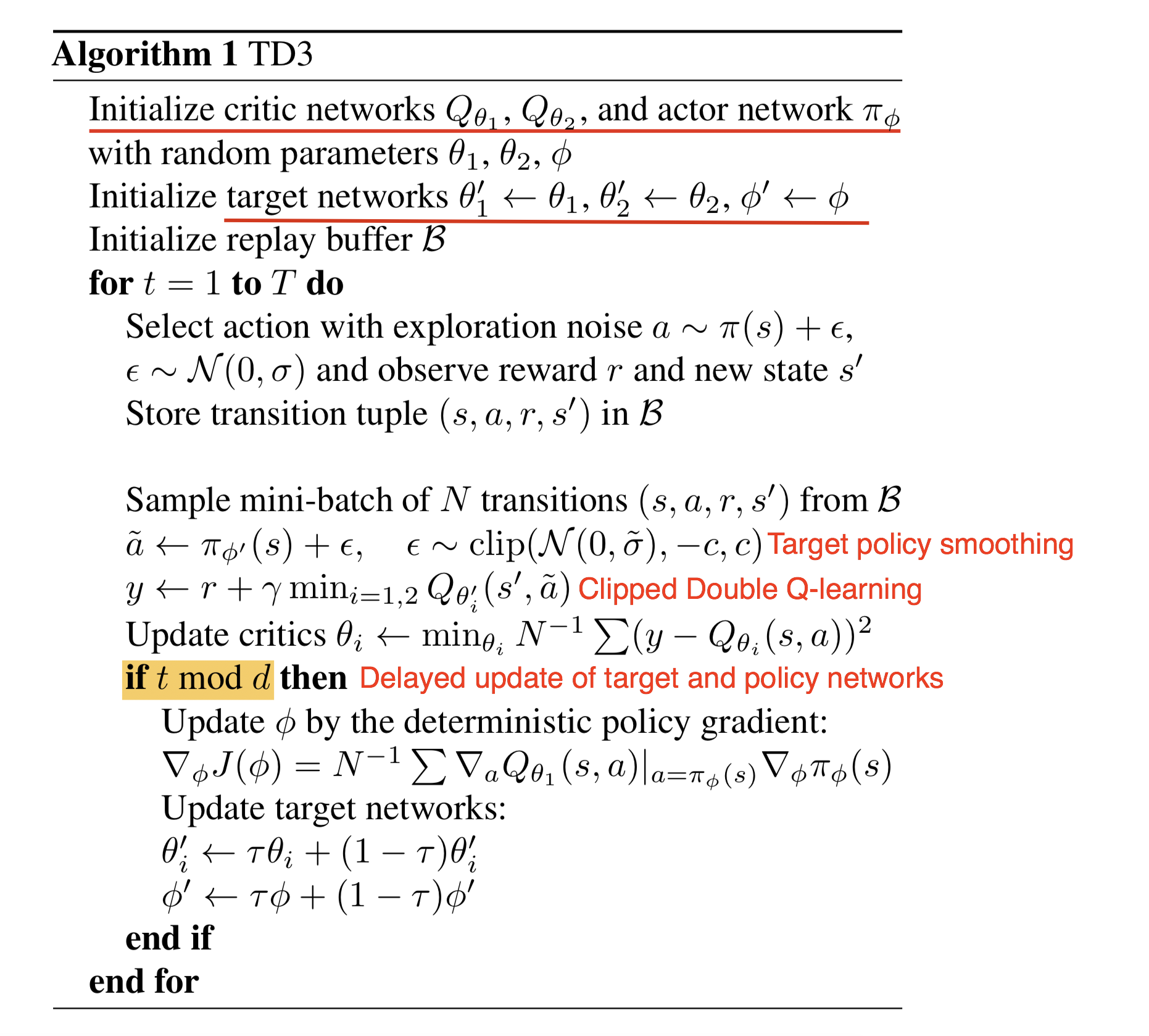
Fig 8. TD3 Algorithm. (Image source: Fujimoto et al., 2018)
SVPG
Stein Variational Policy Gradient (SVPG; Liu et al, 2017) applies the Stein variational gradient descent (SVGD; Liu and Wang, 2016) algorithm to update the policy parameter θθ.
In the setup of maximum entropy policy optimization, θθ is considered as a random variable θ∼q(θ)θ∼q(θ) and the model is expected to learn this distribution q(θ)q(θ). Assuming we know a prior on how qq might look like, q0q0, and we would like to guide the learning process to not make θθ too far away from q0q0 by optimizing the following objective function:
where Eθ∼q[R(θ)]Eθ∼q[R(θ)] is the expected reward when θ∼q(θ)θ∼q(θ) and DKLDKL is the KL divergence.
If we don’t have any prior information, we might set q0q0 as a uniform distribution and set q0(θ)q0(θ) to a constant. Then the above objective function becomes SAC, where the entropy term encourages exploration:
Let’s take the derivative of J^(θ)=Eθ∼q[J(θ)]−αDKL(q∥q0)J^(θ)=Eθ∼q[J(θ)]−αDKL(q‖q0) w.r.t. qq:
The optimal distribution is:
The temperature αα decides a tradeoff between exploitation and exploration. When α→0α→0, θθ is updated only according to the expected return J(θ)J(θ). When α→∞α→∞, θθ always follows the prior belief.
When using the SVGD method to estimate the target posterior distribution q(θ)q(θ), it relies on a set of particle {θi}ni=1{θi}i=1n (independently trained policy agents) and each is updated:
where ϵϵ is a learning rate and ϕ∗ϕ∗ is the unit ball of a RKHS (reproducing kernel Hilbert space) HH of θθ-shaped value vectors that maximally decreases the KL divergence between the particles and the target distribution. q′(.)q′(.) is the distribution of θ+ϵϕ(θ)θ+ϵϕ(θ).
Comparing different gradient-based update methods:
| Method | Update space |
|---|---|
| Plain gradient | ΔθΔθ on the parameter space |
| Natural gradient | ΔθΔθ on the search distribution space |
| SVGD | ΔθΔθ on the kernel function space (edited) |
One estimation of ϕ∗ϕ∗ has the following form. A positive definite kernel k(ϑ,θ)k(ϑ,θ), i.e. a Gaussian radial basis function, measures the similarity between particles.
- The first term in red encourages θiθi learning towards the high probability regions of qq that is shared across similar particles. => to be similar to other particles
- The second term in green pushes particles away from each other and therefore diversifies the policy. => to be dissimilar to other particles
Usually the temperature αα follows an annealing scheme so that the training process does more exploration at the beginning but more exploitation at a later stage.
Quick Summary
After reading through all the algorithms above, I list a few building blocks or principles that seem to be common among them:
- Try to reduce the variance and keep the bias unchanged to stabilize learning.
- Off-policy gives us better exploration and helps us use data samples more efficiently.
- Experience replay (training data sampled from a replay memory buffer);
- Target network that is either frozen periodically or updated slower than the actively learned policy network;
- Batch normalization;
- Entropy-regularized reward;
- The critic and actor can share lower layer parameters of the network and two output heads for policy and value functions.
- It is possible to learn with deterministic policy rather than stochastic one.
- Put constraint on the divergence between policy updates.
- New optimization methods (such as K-FAC).
- Entropy maximization of the policy helps encourage exploration.
- Try not to overestimate the value function.
- TBA more.
Cited as:
@article{weng2018PG,

  title   = "Policy Gradient Algorithms",

  author  = "Weng, Lilian",

  journal = "lilianweng.github.io/lil-log",

  year    = "2018",

  url     = "https://lilianweng.github.io/lil-log/2018/04/08/policy-gradient-algorithms.html"

}
References
[1] jeremykun.com Markov Chain Monte Carlo Without all the Bullshit
[2] Richard S. Sutton and Andrew G. Barto. Reinforcement Learning: An Introduction; 2nd Edition. 2017.
[3] John Schulman, et al. “High-dimensional continuous control using generalized advantage estimation.” ICLR 2016.
[4] Thomas Degris, Martha White, and Richard S. Sutton. “Off-policy actor-critic.” ICML 2012.
[5] timvieira.github.io Importance sampling
[6] Mnih, Volodymyr, et al. “Asynchronous methods for deep reinforcement learning.” ICML. 2016.
[7] David Silver, et al. “Deterministic policy gradient algorithms.” ICML. 2014.
[8] Timothy P. Lillicrap, et al. “Continuous control with deep reinforcement learning.” arXiv preprint arXiv:1509.02971 (2015).
[9] Ryan Lowe, et al. “Multi-agent actor-critic for mixed cooperative-competitive environments.” NIPS. 2017.
[10] John Schulman, et al. “Trust region policy optimization.” ICML. 2015.
[11] Ziyu Wang, et al. “Sample efficient actor-critic with experience replay.” ICLR 2017.
[12] Rémi Munos, Tom Stepleton, Anna Harutyunyan, and Marc Bellemare. “Safe and efficient off-policy reinforcement learning” NIPS. 2016.
[13] Yuhuai Wu, et al. “Scalable trust-region method for deep reinforcement learning using Kronecker-factored approximation.” NIPS. 2017.
[14] kvfrans.com A intuitive explanation of natural gradient descent
[15] Sham Kakade. “A Natural Policy Gradient.”. NIPS. 2002.
[16] “Going Deeper Into Reinforcement Learning: Fundamentals of Policy Gradients.” - Seita’s Place, Mar 2017.
[17] “Notes on the Generalized Advantage Estimation Paper.” - Seita’s Place, Apr, 2017.
[18] Gabriel Barth-Maron, et al. “Distributed Distributional Deterministic Policy Gradients.” ICLR 2018 poster.
[19] Tuomas Haarnoja, Aurick Zhou, Pieter Abbeel, and Sergey Levine. “Soft Actor-Critic: Off-Policy Maximum Entropy Deep Reinforcement Learning with a Stochastic Actor.” arXiv preprint arXiv:1801.01290 (2018).
[20] Scott Fujimoto, Herke van Hoof, and Dave Meger. “Addressing Function Approximation Error in Actor-Critic Methods.” arXiv preprint arXiv:1802.09477 (2018).
[21] Tuomas Haarnoja, et al. “Soft Actor-Critic Algorithms and Applications.” arXiv preprint arXiv:1812.05905 (2018).
[22] David Knowles. “Lagrangian Duality for Dummies” Nov 13, 2010.
[23] Yang Liu, et al. “Stein variational policy gradient.” arXiv preprint arXiv:1704.02399 (2017).
[24] Qiang Liu and Dilin Wang. “Stein variational gradient descent: A general purpose bayesian inference algorithm.” NIPS. 2016.
Policy Gradient Algorithms的更多相关文章
- Deep Learning专栏--强化学习之从 Policy Gradient 到 A3C(3)
在之前的强化学习文章里,我们讲到了经典的MDP模型来描述强化学习,其解法包括value iteration和policy iteration,这类经典解法基于已知的转移概率矩阵P,而在实际应用中,我们 ...
- (转)RL — Policy Gradient Explained
RL — Policy Gradient Explained 2019-05-02 21:12:57 This blog is copied from: https://medium.com/@jon ...
- Ⅶ. Policy Gradient Methods
Dictum: Life is just a series of trying to make up your mind. -- T. Fuller 不同于近似价值函数并以此计算确定性的策略的基于价 ...
- DRL之:策略梯度方法 (Policy Gradient Methods)
DRL 教材 Chpater 11 --- 策略梯度方法(Policy Gradient Methods) 前面介绍了很多关于 state or state-action pairs 方面的知识,为了 ...
- 强化学习(十三) 策略梯度(Policy Gradient)
在前面讲到的DQN系列强化学习算法中,我们主要对价值函数进行了近似表示,基于价值来学习.这种Value Based强化学习方法在很多领域都得到比较好的应用,但是Value Based强化学习方法也有很 ...
- [Reinforcement Learning] Policy Gradient Methods
上一篇博文的内容整理了我们如何去近似价值函数或者是动作价值函数的方法: \[ V_{\theta}(s)\approx V^{\pi}(s) \\ Q_{\theta}(s)\approx Q^{\p ...
- 强化学习--Policy Gradient
Policy Gradient综述: Policy Gradient,通过学习当前环境,直接给出要输出的动作的概率值. Policy Gradient 不是单步更新,只能等玩完一个epoch,再 ...
- 深度学习课程笔记(十三)深度强化学习 --- 策略梯度方法(Policy Gradient Methods)
深度学习课程笔记(十三)深度强化学习 --- 策略梯度方法(Policy Gradient Methods) 2018-07-17 16:50:12 Reference:https://www.you ...
- 论文笔记之:SeqGAN: Sequence generative adversarial nets with policy gradient
SeqGAN: Sequence generative adversarial nets with policy gradient AAAI-2017 Introduction : 产生序列模拟数 ...
随机推荐
- consul:健康检查
官方文档:https://www.consul.io/docs/agent/checks.html consul提供的健康检查有以下几种: 1.script+interval 2.http+inter ...
- pandas 之 索引重塑
import numpy as np import pandas as pd There are a number of basic operations for rearanging tabular ...
- python语言的堆栈与队列类的实现
基于python语言的数据结构之堆栈与队列的实现 # 堆栈的实现 # -*- coding: utf-8 -*- """ 栈(stack), 是一种容器,可以存入数据元素 ...
- linux cgroups简介(上)
Linux CGroups简介 1.CGroups是什么 与Linux namespace对比来看,Linux namespace用来限制进程的运行范围或者运行环境的可见性,比如:uts限制进程读取到 ...
- ShortKey – Visual Studio/VS Code etc.
Switching between .h and .cppIn Visual Studio 2013 and later :there is a default keyboard shortcut f ...
- php7新增的两个操作符---null合并及飞船操作符
<?php //null合并操作符?? //(太空)飞船操作符<=> //The operator returns 0 if both operands are equal, 1 i ...
- 安卓QQ聊天记录导出、备份完全攻略
发到知乎竟然被删掉,我也不知道我到底违反了哪条.唉,别人的毕竟是别人的.虽然博客园也是别人的 前言 我对聊天记录的备份比较执着,也在这上面折腾过不少.碰到过不少令人头疼的麻烦,在这里分享一下经验. 关 ...
- C#多线程编程中的锁系统
C#多线程编程中的锁系统(二) 上章主要讲排他锁的直接使用方式.但实际当中全部都用锁又太浪费了,或者排他锁粒度太大了. 这一次我们说说升级锁和原子操作. 目录 1:volatile 2: Inter ...
- destoon开发笔记-JQ+JS实现倒计时功能
页面代码 <div class="time " class="" id="onBidtime125" pid="125&qu ...
- Maven pom文件中dependency scope用法
在Maven中依赖的域有:compile.provided.runtime.system.test.import 一.compile(默认) 当依赖的scope为compile的时候,那么当前这个依赖 ...
