Exercise:Sparse Autoencoder

斯坦福deep learning教程中的自稀疏编码器的练习，主要是参考了   http://www.cnblogs.com/tornadomeet/archive/2013/03/20/2970724.html，没有参考肯定编不出来。。。Σ( ° △ °|||)︴  也当自己理解了一下

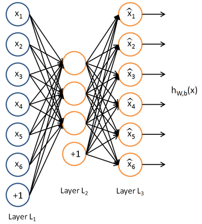
这里的自稀疏编码器，练习上规定是64个输入节点，25个隐藏层节点（我实验中只有20个），输出层也是64个节点，一共有10000个训练样本

具体步骤：

首先在页面上下载sparseae_exercise.zip

Step 1：构建训练集

要求在10张图片（图片数据存储在IMAGES中）中随机的选取一张图片，在再这张图片中随机的选取10000个像素点，最终构建一个64*10000的像素矩阵。从一张图片中选取10000个像素点的好处是，只有copy一次IMAGES，速度更快，但是要注意每张图片的像素是512*512的，所以随机选取像素点最好是分行和列各选取100，最终组合成100*100，这样不容易导致越界。验证step 1可以运行train.m中的第一步，结果图如下：

（只展示了200个sample，所以有4个缺口）

需要自行编写sampleIMAGES中的部分code

function patches = sampleIMAGES()
% sampleIMAGES
% Returns  patches for training

load IMAGES;    % load images from disk 

patchsize = ;  % we'll use 8x8 patches
numpatches = ;

% Initialize patches with zeros.  Your code will fill in this matrix--one
% column per patch,  columns.
patches = zeros(patchsize*patchsize, numpatches);

%% ---------- YOUR CODE HERE --------------------------------------
%  Instructions: Fill in the variable called "patches" using data
%  from IMAGES.
%
%  IMAGES is a 3D array containing  images
%  For instance, IMAGES(:,:,) is a 512x512 array containing the 6th image,
%  and you can type "imagesc(IMAGES(:,:,6)), colormap gray;" to visualize
%  it. (The contrast on these images look a bit off because they have
%  been preprocessed using using "whitening."  See the lecture notes for
%  more details.) As a second example, IMAGES(:,:,) is an image
%  patch corresponding to the pixels in the block (,) to (,) of
%  Image 

imageNum = randi([,]);     %随机的选择一张图片
[rowNum colNum] = size(IMAGES(:,:,imageNum));
xPos = randperm(rowNum-patchsize+,);
yPos = randperm(colNum-patchsize+,);
for ii = :                %在图片中选取100*100个像素点
    for jj = :
        patchNum = (ii-)* + jj;
        patches(:,patchNum) = reshape(IMAGES(xPos(ii):xPos(ii)+,yPos(jj):yPos(jj)+,...
                                      imageNum),,);
    end
end

%% ---------------------------------------------------------------
% For the autoencoder to work well we need to normalize the data
% Specifically, since the output of the network is bounded between [,]
% (due to the sigmoid activation function), we have to make sure
% the range of pixel values is also bounded between [,]
patches = normalizeData(patches);

end

%% ---------------------------------------------------------------
function patches = normalizeData(patches)

% Squash data to [0.1, 0.9] since we use sigmoid as the activation
% function in the output layer

% Remove DC (mean of images).
patches = bsxfun(@minus, patches, mean(patches));

% Truncate to +/- standard deviations and scale to - to
pstd =  * std(patches(:));
patches = max(min(patches, pstd), -pstd) / pstd;

% Rescale from [-,] to [0.1,0.9]
patches = (patches + ) * 0.4 + 0.1;

end

Step 2：求解自稀疏编码器的参数

这一步就是要运用BP算法求解NN中各层的W，b（W1，W2，b1，b2）参数。 Backpropagation Algorithm算法在教程的第二节中有介绍，但要注意的是自稀疏编码器的误差函数除了有参数的正则化项，还有稀疏性规则项，BP算法推导公式中要加上，这里需要自行编写sparseAutoencoderCost.m

function [cost,grad] = sparseAutoencoderCost(theta, visibleSize, hiddenSize, ...
                                             lambda, sparsityParam, beta, data)

% visibleSize: the number of input units (probably )
% hiddenSize: the number of hidden units (probably )
% lambda: weight decay parameter
% sparsityParam: The desired average activation for the hidden units (denoted in the lecture
%                           notes by the greek alphabet rho, which looks like a lower-case "p").
% beta: weight of sparsity penalty term
% data: Our 64x10000 matrix containing the training data.  So, data(:,i) is the i-th training example. 

% The input theta is a vector (because minFunc expects the parameters to be a vector).
% We first convert theta to the (W1, W2, b1, b2) matrix/vector format, so that this
% follows the notation convention of the lecture notes. 

W1 = reshape(theta(:hiddenSize*visibleSize), hiddenSize, visibleSize);
W2 = reshape(theta(hiddenSize*visibleSize+:*hiddenSize*visibleSize), visibleSize, hiddenSize);
b1 = theta(*hiddenSize*visibleSize+:*hiddenSize*visibleSize+hiddenSize);
b2 = theta(*hiddenSize*visibleSize+hiddenSize+:end);

% Cost and gradient variables (your code needs to compute these values).
% Here, we initialize them to zeros.
cost = ;
W1grad = zeros(size(W1));
W2grad = zeros(size(W2));
b1grad = zeros(size(b1));
b2grad = zeros(size(b2));

%% ---------- YOUR CODE HERE --------------------------------------
%  Instructions: Compute the cost/optimization objective J_sparse(W,b) for the Sparse Autoencoder,
%                and the corresponding gradients W1grad, W2grad, b1grad, b2grad.
%
% W1grad, W2grad, b1grad and b2grad should be computed using backpropagation.
% Note that W1grad has the same dimensions as W1, b1grad has the same dimensions
% as b1, etc.  Your code should set W1grad to be the partial derivative of J_sparse(W,b) with
% respect to W1.  I.e., W1grad(i,j) should be the partial derivative of J_sparse(W,b)
% with respect to the input parameter W1(i,j).  Thus, W1grad should be equal to the term
% [(/m) \Delta W^{()} + \lambda W^{()}] in the last block of pseudo-code in Section 2.2
% of the lecture notes (and similarly for W2grad, b1grad, b2grad).
%
% Stated differently, if we were using batch gradient descent to optimize the parameters,
% the gradient descent update to W1 would be W1 := W1 - alpha * W1grad, and similarly for W2, b1, b2.
% 

Jcost = ;%直接误差
Jweight = ;%权值惩罚
Jsparse = ;%稀疏性惩罚
[n m] = size(data);%m为样本的个数，n为样本的特征数

%前向算法计算各神经网络节点的线性组合值和active值
z2 = W1*data+repmat(b1,,m);%注意这里一定要将b1向量复制扩展成m列的矩阵
a2 = sigmoid(z2);
z3 = W2*a2+repmat(b2,,m);
a3 = sigmoid(z3);

% 计算预测产生的误差
Jcost = (0.5/m)*sum(sum((a3-data).^));

%计算权值惩罚项
Jweight = (/)*(sum(sum(W1.^))+sum(sum(W2.^)));

%计算稀释性规则项
rho = (/m).*sum(a2,)  ;%求出第一个隐含层的平均值向量
Jsparse = sum(sparsityParam.*log(sparsityParam./rho)+ ...
        (-sparsityParam).*log((-sparsityParam)./(-rho)));

%损失函数的总表达式
cost = Jcost+lambda*Jweight+beta*Jsparse;

%反向算法求出每个节点的误差值
d3 = -(data-a3).*(a3.*(-a3));
sterm = beta*(-sparsityParam./rho+(-sparsityParam)./(-rho));%因为加入了稀疏规则项，所以
                                                             %计算偏导时需要引入该项
d2 = (W2'*d3+repmat(sterm,1,m)).*(a2.*(1-a2)); 

%计算W1grad
W1grad = W1grad+d2*data';
W1grad = (/m)*W1grad+lambda*W1;

%计算W2grad
W2grad = W2grad+d3*a2';
W2grad = (/m).*W2grad+lambda*W2;

%计算b1grad
b1grad = b1grad+sum(d2,);
b1grad = (/m)*b1grad;%注意b的偏导是一个向量，所以这里应该把每一行的值累加起来

%计算b2grad
b2grad = b2grad+sum(d3,);
b2grad = (/m)*b2grad;

%-------------------------------------------------------------------
% After computing the cost and gradient, we will convert the gradients back
% to a vector format (suitable for minFunc).  Specifically, we will unroll
% your gradient matrices into a vector.

grad = [W1grad(:) ; W2grad(:) ; b1grad(:) ; b2grad(:)];

end

%-------------------------------------------------------------------
% Here's an implementation of the sigmoid function, which you may find useful
% in your computation of the costs and the gradients.  This inputs a (row or
% column) vector (say (z1, z2, z3)) and returns (f(z1), f(z2), f(z3)). 

function sigm = sigmoid(x)        % 定义sigmoid函数

    sigm =  ./ ( + exp(-x));
end

Step 3：求解的 梯度检验

验证梯度下降是否正确，这个在教程第三节也有介绍，比较简单，在computeNumericalGradient.m中返回梯度检验后的值即可，computeNumericalGradient.m是在checkNumericalGradient.m中调用的，而checkNumericalGradient.m已经给出，不需要我们自己编写。

function numgrad = computeNumericalGradient(J, theta)
% numgrad = computeNumericalGradient(J, theta)
% theta: a vector of parameters
% J: a function that outputs a real-number. Calling y = J(theta) will return the
% function value at theta. 

% Initialize numgrad with zeros
numgrad = zeros(size(theta));

%% ---------- YOUR CODE HERE --------------------------------------
% Instructions:
% Implement numerical gradient checking, and return the result in numgrad.
% (See Section 2.3 of the lecture notes.)
% You should write code so that numgrad(i) is (the numerical approximation to) the
% partial derivative of J with respect to the i-th input argument, evaluated at theta.
% I.e., numgrad(i) should be the (approximately) the partial derivative of J with
% respect to theta(i).
%
% Hint: You will probably want to compute the elements of numgrad one at a time. 

epsilon = 1e-;
n = size(theta,);
E = eye(n,1);
for i = :n
　　 E(i) = 1;
    delta = E*epsilon;
    numgrad(i) = (J(theta+delta)-J(theta-delta))/(epsilon*2.0);
　　 E(i) = 0;
end

%% ---------------------------------------------------------------
end

Step 4：训练自稀疏编码器

整个训练过程使用的是L-BFGS求解，比教程中介绍的主要介绍批量SGD要快很多，具体原理我也不知道，而且训练过程已经给出，这一段不需要我们自己编写

Step 5：输出可视化结果

训练结束后，输出训练得到的权重矩阵W1，结果同时也会保存在weights.jpg中，这一段也不需要我们编写（ 第一次）

结果图如下：

（感觉自己训练出来的这个没有标准的那么明显的线条，看就了还有点类似错误示例的第3个，不过重新仔细看还是有线条感的，可能是因为隐藏层只有20个，训练的也没有25个的彻底）

另外，查了一下内存不足的解决方法，据说在matlab命令行输入pack，可以释放一些内存。但是我觉得还是终究治标不治本，最好的方法还是升级64位操作系统，去添加内存条吧~

剩下的.m文件都不需要我们自己编写（修改隐藏层的节点数在train.m中），不过也顺带附上吧

function [] = checkNumericalGradient()
% This code can be used to check your numerical gradient implementation
% in computeNumericalGradient.m
% It analytically evaluates the gradient of a very simple function called
% simpleQuadraticFunction (see below) and compares the result with your numerical
% solution. Your numerical gradient implementation is incorrect if
% your numerical solution deviates too much from the analytical solution.

% Evaluate the function and gradient at x = [; ]; (Here, x is a 2d vector.)
x = [; ];
[value, grad] = simpleQuadraticFunction(x);

% Use your code to numerically compute the gradient of simpleQuadraticFunction at x.
% (The notation "@simpleQuadraticFunction" denotes a pointer to a function.)
numgrad = computeNumericalGradient(@simpleQuadraticFunction, x);

% Visually examine the two gradient computations.  The two columns
% you get should be very similar.
disp([numgrad grad]);
fprintf('The above two columns you get should be very similar.\n(Left-Your Numerical Gradient, Right-Analytical Gradient)\n\n');

% Evaluate the norm of the difference between two solutions.
% If you have a correct implementation, and assuming you used EPSILON = 0.0001
% in computeNumericalGradient.m, then diff below should be 2.1452e-12
diff = norm(numgrad-grad)/norm(numgrad+grad);
disp(diff);
fprintf('Norm of the difference between numerical and analytical gradient (should be < 1e-9)\n\n');
end

function [value,grad] = simpleQuadraticFunction(x)
% this function accepts a 2D vector as input.
% Its outputs are:
%   value: h(x1, x2) = x1^ + *x1*x2
%   grad: A 2x1 vector that gives the partial derivatives of h with respect to x1 and x2
% Note that when we pass @simpleQuadraticFunction(x) to computeNumericalGradients, we're assuming
% that computeNumericalGradients will use only the first returned value of this function.

value = x()^ + *x()*x();

grad = zeros(, );
grad()  = *x() + *x();
grad()  = *x();

end

checkNumericalGradient.m

function theta = initializeParameters(hiddenSize, visibleSize)

%% Initialize parameters randomly based on layer sizes.
r  = sqrt() / sqrt(hiddenSize+visibleSize+);   % we'll choose weights uniformly from the interval [-r, r]
W1 = rand(hiddenSize, visibleSize) *  * r - r;
W2 = rand(visibleSize, hiddenSize) *  * r - r;

b1 = zeros(hiddenSize, );
b2 = zeros(visibleSize, );

% Convert weights and bias gradients to the vector form.
% This step will "unroll" (flatten and concatenate together) all
% your parameters into a vector, which can then be used with minFunc.
theta = [W1(:) ; W2(:) ; b1(:) ; b2(:)];

end

initializeParameter

function [h, array] = display_network(A, opt_normalize, opt_graycolor, cols, opt_colmajor)

% This function visualizes filters in matrix A. Each column of A is a
% filter. We will reshape each column into a square image and visualizes
% on each cell of the visualization panel.
% All other parameters are optional, usually you do not need to worry
% about it.
% opt_normalize: whether we need to normalize the filter so that all of
% them can have similar contrast. Default value is true.
% opt_graycolor: whether we use gray as the heat map. Default is true.
% cols: how many columns are there in the display. Default value is the
% squareroot of the number of columns in A.
% opt_colmajor: you can switch convention to row major for A. In that
% case, each row of A is a filter. Default value is false.
warning off all

if ~exist('opt_normalize', 'var') || isempty(opt_normalize)
    opt_normalize= true;
end

if ~exist('opt_graycolor', 'var') || isempty(opt_graycolor)
    opt_graycolor= true;
end

if ~exist('opt_colmajor', 'var') || isempty(opt_colmajor)
    opt_colmajor = false;
end

% rescale
A = A - mean(A(:));

if opt_graycolor, colormap(gray); end

% compute rows, cols
[L M]=size(A);
sz=sqrt(L);
buf=;
if ~exist('cols', 'var')
    if floor(sqrt(M))^ ~= M
        n=ceil(sqrt(M));
        while mod(M, n)~= && n<1.2*sqrt(M), n=n+; end
        m=ceil(M/n);
    else
        n=sqrt(M);
        m=n;
    end
else
    n = cols;
    m = ceil(M/n);
end

array=-ones(buf+m*(sz+buf),buf+n*(sz+buf));

if ~opt_graycolor
    array = 0.1.* array;
end

if ~opt_colmajor
    k=;
    for i=:m
        for j=:n
            if k>M,
                continue;
            end
            clim=max(abs(A(:,k)));
            if opt_normalize
                array(buf+(i-)*(sz+buf)+(:sz),buf+(j-)*(sz+buf)+(:sz))=reshape(A(:,k),sz,sz)/clim;
            else
                array(buf+(i-)*(sz+buf)+(:sz),buf+(j-)*(sz+buf)+(:sz))=reshape(A(:,k),sz,sz)/max(abs(A(:)));
            end
            k=k+;
        end
    end
else
    k=;
    for j=:n
        for i=:m
            if k>M,
                continue;
            end
            clim=max(abs(A(:,k)));
            if opt_normalize
                array(buf+(i-)*(sz+buf)+(:sz),buf+(j-)*(sz+buf)+(:sz))=reshape(A(:,k),sz,sz)/clim;
            else
                array(buf+(i-)*(sz+buf)+(:sz),buf+(j-)*(sz+buf)+(:sz))=reshape(A(:,k),sz,sz);
            end
            k=k+;
        end
    end
end

if opt_graycolor
    h=imagesc(array,'EraseMode','none',[- ]);
else
    h=imagesc(array,'EraseMode','none',[- ]);
end
axis image off

drawnow;

warning on all

display_network