深度学习原理与框架-图像补全(原理与代码) 1.tf.nn.moments(求平均值和标准差) 2.tf.control_dependencies(先执行内部操作) 3.tf.cond(判别执行前或后函数) 4.tf.nn.atrous_conv2d 5.tf.nn.conv2d_transpose(反卷积) 7.tf.train.get_checkpoint_state(判断sess是否存在

1. tf.nn.moments(x, axes=[0, 1, 2])  # 对前三个维度求平均值和标准差，结果为最后一个维度，即对每个feature_map求平均值和标准差

参数说明：x为输入的feature_map, axes=[0, 1, 2] 对三个维度求平均，即每一个feature_map都获得一个平均值和标准差

2.with tf.control_dependencies([train_mean, train_var])： 即执行with里面的操作时，会先执行train_mean 和 train_var

参数说明：train_mean表示对pop_mean进行赋值的操作，train_var表示对pop_var进行赋值的操作

3.tf.cond(is_training, bn_train, bn_inference)  # 如果is_training为真，执行bn_train函数操作，如果为假，执行bn_inference操作

参数说明：is_training 为真和假，bn_train表示训练的normalize， bn_inference表示测试的normalize

4. tf.nn.atrous_conv2d(x, filters, dilated, padding) # 进行空洞卷积操作，用于增加卷积的感受野

参数说明：x表示输入样本，filter表示卷积核，dilated表示卷积核的补零个数，padding表示对feature进行补零操作

5. tf.nn.conv2d_transpose(x, filters, output_size, strides) # 进行反卷积操作

参数说明：x表示输入样本，filter表示卷积核，output_size表示输出的维度， strides表示图像扩大的倍数

6.tf.nn.batch_normalization(x, mean, var, beta, scale, episilon) # 进行归一化操作

参数说明： x表示输入样本，mean表示卷积的平均值，var表示卷积的标准差，beta表示偏差，scale表示标准化后的范围，episilon防止分母为0

7.tf.train.get_checkpoint_state('./backup') # 判断用于进行model保存的文件中是否有checkpoint，即是否之前已经有过保存的sess

参数说明：'./backup'进行sess保存的文件名

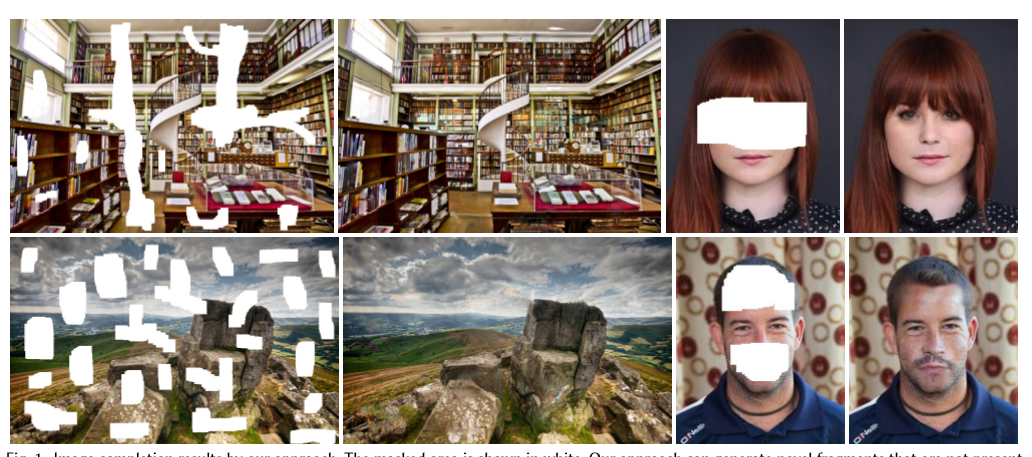
原理的话,使用论文中的图进行说明， 这是论文中的效果图，我们可以看出不管是场景还是人脸都有较好的复原效果

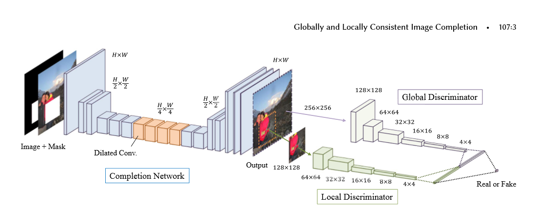
下面是论文的结构图， 主要是有2个结构组成，

第一个结构是全卷机填充网络：首先使用一个mask和图片进行组合，构成了具有空缺的图片，将空缺图片输入到全卷积中，经过stride等于2，做两次的向下卷积，然后经过4个dilated_conv(空洞卷积)，为了在不损失维度的情况下，增加卷积核的视野，最后使用补零的反转卷积进行维度的升高，再经过最后两层卷积构成了图片。

第二个结构是global_discrimanator 和 local_discimanator

对于global_x输入的大小为全图的大小，而local_x的输入大小为全图大小的一半，上图的mask的大小为96-128且在local_x的内部，取值的范围为随机值

global_x 和 local_x经过卷积后，输出1024的输出，我们将输出进行串接tf.concat，对最后的输出结果[1]进行预测,判别图片为实际图片(真)还是经过填充的图片(假)

网络系数的展示

      

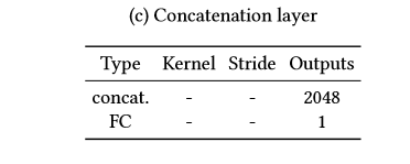
填充网络(卷积-空洞卷积-反卷积)                     全局判别网络(卷积-全连接)                                局部判别网络(卷积-全连接)               串接网络(全连接)

训练步骤：为了使得对抗网络训练更加的有效，我们需要先对填充网络进行预训练，然后是对判别网络进行训练，最后将生成网络和判别网络放在一起进行训练

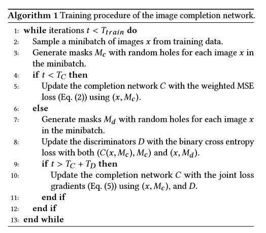
这里说明一下，填充 网络的损失值是mse，即tf.l2_loss()  判别网络的损失值是tf.reduce_mean(tf.nn.softmax...logits)

代码：代码主要由五个.py文件构建，

1.to_npy进行图片的预处理，并将数据保存为.npy文件，

2.load.py 使用np.load进行x_train和x_test数据的读取

3.train.py 主要进行参数的训练，并且构造出mask_batch, local_x和local_complement

4.network用于进行模型结构的搭建，构建生成网络和判别网络，同时获得生成网络和判别网络的损失值

5.layer 用于卷积，反卷积，全连接，空洞卷积等函数的构建

数据的准备：to_npy

import numpy as np
import tensorflow as tf
import glob
import cv2
import os
 
# 将处理好的图片进行保存，为了防止经常需要处理图片
# 进行数据的压缩
IMAGE_SIZE = 128
# 训练集的比例
train_ep = 0.9
x = []
# 循环文件中的所有图片的地址
pathes = glob.glob('/data/*jpg')
# 循环前500个图片的地址
for path in pathes[:500]:
    # 使用cv2.imread读取图片
    img = cv2.imread(path)
    # 将图片进行维度的变换
    img = cv2.resize(img, (IMAGE_SIZE, IMAGE_SIZE))
    # 将读入的图片从BGR转换为RGB
    img = cv2.cvtColor(img, cv2.COLOR_BGR2RGB)
    # 将图片添加到列表中
    x.append(img)
# 如果不存在./npy文件
if not os.path.exists('./npy'):
    # 使用os.makedirs进行创建文件npy
    os.makedirs('./npy')
 
# 获得train的索引
p = len(x) * train_ep
# 训练集x
train_x = x[:p]
# 测试集x
test_x = x[p:]
# 将预处理好的图片保存为.npy文件
np.save('./npy/x_train.npy', train_x)
np.save('./npy/x_test.npy', test_x)

train.py

import numpy as np
import tensorflow as tf
import os
from network import *
import load
import tqdm
import cv2
 
# 第一步：定义超参数
IMAGE_SIZE = 128  # 输入图片的大小
LOCAL_SIZE = 64   # local的大小
HOL_MIN = 24     # 洞的最小值
HOL_MAX = 48     # 洞的最大值
LEARNING_RATE = 1e-3 # 学习率
BATCH_SIZE = 1   # batch_size大小
PRETRAIN_NUM = 100  # 对生成网络预训练的次数
 
def train():
    # 第二步：构造输入的初始化参数
    x = tf.placeholder(tf.float32, [BATCH_SIZE, IMAGE_SIZE, IMAGE_SIZE, 3]) # 图片x，维度为1, 128, 128, 3
    mask = tf.placeholder(tf.float32, [BATCH_SIZE, IMAGE_SIZE, IMAGE_SIZE, 1]) # 掩模mask, 1, 128, 128, 1用于生成图片空白区域
    x_local = tf.placeholder(tf.float32, [BATCH_SIZE, LOCAL_SIZE, LOCAL_SIZE, 3]) # 图片x部分图像，维度为1, 64, 64, 3
    completion_global = tf.placeholder(tf.float32, [BATCH_SIZE, IMAGE_SIZE, IMAGE_SIZE, 3]) # 生成图像的维度，1， 128，128，3
    completion_local = tf.placeholder(tf.float32, [BATCH_SIZE, LOCAL_SIZE, LOCAL_SIZE, 3]) # 生成图像部分图像，1, 64, 64, 3
    is_training = tf.placeholder(tf.bool, []) # 是够进行训练，在batch_normalize中使用
 
    # 第三步：调用network,构造网络框架，包括生成网络，判别网络，以及其生成和判别的损失值
    model = Network(x, mask, x_local, completion_global, completion_local, is_training, BATCH_SIZE)
 
    # 第四步：使用tf.session 构造sess
    sess = tf.Session()
 
    # 第五步：初始化global_step和epoch
    global_step = tf.Variable(0, name='global_step', trainable=False)
    epoch = tf.Variable(0, name='epoch', trainable=False)
    # 第六步：构造自适应梯度下降器，获得生成网络和判别网络损失值下降操作
    opt = tf.train.AdamOptimizer(LEARNING_RATE)
    g_loss_op = opt.minimize(model.g_loss, global_step=global_step)
    d_loss_op = opt.minimize(model.d_loss, global_step=global_step)
    # 第七步：使用sess.run进行初始化操作
    init = tf.global_variables_initializer()
    sess.run(init)
    # 第八步：如果存在./backup文件，就使用saver.restore()加载sess
    if tf.train.get_checkpoint_state('./backup'):
        saver = tf.train.Saver()
        saver.restore(sess, './backup/latest')
    # 第九步：获得训练集和测试集，使用load中定义的load函数， 并对读取的图片做归一化操作
    x_train, x_test = load.load()
    x_train = np.array([a/127.5 - 1 for a in x_train])
    x_test = np.array([a/127.5 - 1 for a in x_test])
    # 定义一个epoch迭代的次数
    step_num = int(len(x_train)/BATCH_SIZE)
 
    while True:
        # 第十步：将epoch值进行+1操作
        sess.run(tf.assign_add(epoch, 1))
        # 对输入的x_train进行洗牌操作，每次迭代
        np.random.shuffle(x_train)
        # 第十一步：如果当前迭代的次数小于预训练，进行生成网络的训练
        if sess.run(epoch) <= PRETRAIN_NUM:
            # 迭代每个epoch，每次迭代的大小为一个batch_size
            for i in tqdm.tqdm(range(step_num)):
                # 获得一个batch_size的图片
                x_batch = x_train[BATCH_SIZE*i:(i+1)*BATCH_SIZE]
                # 获得points_batch, 和一个batch_size的掩模
                points_batch, masks_batch = get_points()
               # 将x和mask_batch,is_training 传入，进行g_loss_op即损失值的降低
                _, _g_loss = sess.run([g_loss_op, model.g_loss], feed_dict={x:x_batch, mask:masks_batch, is_training:True})
            # 进行验证操作
            # 对x_test进行洗牌操作
            np.random.shuffle(x_test)
            # 获得一个BATHC_SIZE的大小
            x_batch = x_test[:BATCH_SIZE]
            # 获得一个batch_size 的生成图片，执行model.completion
            completion = sess.run([model.completion], feed_dict={x:x_batch, mask:masks_batch, is_training:False})
            # 取出其中一张图片，做归一化的反操作，还原回原始图片
            sample = np.array((completion[0] + 1) * 127.5, dtype=np.uint8)
            # 将图片进行保存，使用cv2.imwrite
            cv2.imwrite('{}_epoch.jpg'.format('{0:06d}'.format(epoch)), cv2.cvtColor(sample, cv2.COLOR_RGB2BGR))
            # 将参数保存在./backup/latest
            saver = tf.train.Saver()
            saver.save(sess, './backup/latest', write_meta_graph=False)
            # 如果次数为100次，就将参数保存在/backup/pre_train
            if sess.run(epoch) == PRETRAIN_NUM:
                saver.save(sess, './backup/pre_train', write_meta_graph=False)
 
        # 第十二步：如果epoch大于预训练的次数，就对生成网络和判别网络进行同时的训练
        else:
            # 循环一个epoch
            for i in tqdm.tqdm(range(step_num)):
                # 获得一个batch的图片
                x_batch = x_train[BATCH_SIZE*i:(i+1)*BATCH_SIZE]
                # 获得一个batch的点坐标，和一个batch的掩模
                points_batch, masks_batch = get_points()
                # 初始化g_loss
                g_loss_value = 0
                # 初始化d_loss
                d_loss_value = 0
                # 执行g_loss_op降低g_loss损失值，同时执行self.completion,获得生成图片completion
                _, completion, g_loss = sess.run([g_loss_op, model.completion, model.g_loss], feed_dict={x:x_batch, mask:masks_batch, is_training:True})
                # 将g_loss添加到g_loss_value
                g_loss_value += g_loss
                # 构造一个batch的x_local
                x_local_batch = []
                # 构造一个batch的completion_batch
                completion_local_batch = []
                # 循环batch_size
                for i in range(BATCH_SIZE):
                    # 获得point_batch中一个点坐标
                    x1, y1, x2, y2 = points_batch[i]
                    # 构造一个x_local, 添加到x_local_batch
                    x_local_batch.append(x_batch[i][y1:y2, x1:x2, :])
                    # 构造一个completion_local, 添加到completion_local_batch
                    completion_local_batch.append(completion[i][y1:y2, x1:x2])
                # 执行d_loss_op，降低d_loss的损失值
                _, d_loss = sess.run([d_loss_op, model.d_loss], feed_dict={x:x_batch, mask:masks_batch, x_local:x_local_batch, completion_global:completion,
                                                                        completion_local:completion_local_batch, is_training:True})
                # 将损失值进行添加
                d_loss_value += d_loss
            # 清洗x_test
            np.random.shuffle(x_test)
            # 获得一个x_batch
            x_batch = x_test[:BATCH_SIZE]
            # 输入测试图片获得生成图片
            completion = sess.run([model.completion], feed_dict={x:x_batch, mask:masks_batch, is_training:False})
            # 取生成图片的第一张图片，进行反归一化
            sample = np.array((completion[0] + 1) * 127.5, dtype=np.uint8)
            # 使用cv2.imwrite保存图片
            cv2.imwrite('{}.epoch'.format('{0:06d}'.format(epoch)), cv2.cvtColor(sample, cv2.COLOR_RGB2BGR))
            # 构造tf.train.Saver() 进行sess的保存操作
            saver = tf.train.Saver()
            saver.save(sess, './backup/latest', write_meta_graph=False)
 
def get_points():
    # 构造点列表，用于构建局部图像
    points = []
    # 构造掩模列表，用于构造残缺的原始图像
    maskes = []
    for i in range(BATCH_SIZE):
        # 获得左上角两个点，范围为[0, IMAGE_SIZE-LOCAL_SIZE]
        x1, y1 = np.random.randint(0, IMAGE_SIZE-LOCAL_SIZE, 2)
        # 获得右下角的两个点，分别进行相加操作
        x2, y2 = np.array([x1, y1]) + LOCAL_SIZE
        # 将坐标添加到points
        points.append([x1, y1, x2, y2])
        # 在H0L_MIN和HOL_MAX范围内构造w，h
        w, h = np.random.randint(HOL_MIN, HOL_MAX, 2)
        # 左上角x轴的坐标为x1+(0, LOCAL_SIZE-w)的范围内
        p1 = x1 + np.random.randint(0, LOCAL_SIZE-w)
        # 左上角y轴的坐标为y1+(0, LOCAL_SIZE-h)的范围内
        q1 = y1 + np.random.randint(0, LOCAL_SIZE-h)
        # 右边的x坐标为p1+w
        p2 = p1 + w
        # 右边的y坐标为q1+h
        q2 = q1 + h
        # 构造全为0的3维矩阵
        m = np.zeros(shape=[IMAGE_SIZE, IMAGE_SIZE, 1])
        # 在该范围内的值为1， 并进行添加
        m[q1:q2, p1:p2, :] = 1
        maskes.append(m)
    # 返回points和掩模的数组
    return np.array(points), np.array(maskes)
 
if __name__ == '__main__':
    train()

代码：network.py： 构建Network类，构造生成网络，生成self.completion, 构造判别网络，获得x,x_local的输出结果self.real，获得global_completion, local_completion的输出结果self.fake, 使用l2_loss构造生成网络的损失值g_loss, 使用交叉熵构造判别网络的损失值d_loss

第一步：使用self.generator构造生成网络， 输入为x*(1-mask), is_training

第二步：使用self.imition * mask + x * (1-mask) 构造self.completion 即生成的图片

第三步：使用self.discrimator, 输入为x, x_local, is_training, reuse=False, 用于真实样本的判别self.real

第四步：使用self.discrimator, 输入为global_complement, local_complement, is_training, reuse=True, 用于生成样本的判别self.fake

第五步：使用tf.nn.l2_loss生成mse的损失值，用于生成网络的损失值，self.g_loss

第六步：使用tf.reduce_mean(tf.sotfmax..logits(labels=tf.ones_like(real), logits=real)) 获得真实的交叉熵，同理获得生成样本的交叉熵，将两者进行加和乘以系数，获得最终的损失值即self.d_loss。

第七步：使用tf.get_collection(tf.GraphKey.TRAINABEL_VARIABLES, scope=‘generator’) 和scope = ‘discrimator’获得生成网络和判别网络的参数

import tensorflow as tf
import numpy as np
from layer import *
 
class Network:
 
    def __init__(self, x, mask, x_local, completion_global, completion_local, is_training, batch_size):
        self.batch_size = batch_size
       # 第一步： 构造生成网络，获得生成的图片，(1-mask) * x 构成残缺空白的输入图片
        self.imition = self.generator((1-mask)*x, is_training)
        # 第二步：将生成图片部分区域与残缺空白的输入图片进行拼接，获得最终的图片
        self.completion = mask * self.imition + (1-mask)*x
        # 第三步：定义discriminator，对x和x_local判断real结果
        self.real = self.discrimator(x, x_local, is_training, reuse=False)
        # 第四步：使用discrimanator,对completion_global 和 completion_local判断fake结果
        self.fake = self.discrimator(completion_global, completion_local, is_training, reuse=True)
        # 第五步：定义生成网络的损失值，使用mse
        self.g_loss = self.cal_g_loss(x, self.completion)
        # 第六步：定义判别网络的损失值，使用交叉熵, 即real判别为1，fake判别为0
        self.d_loss = self.cal_d_loss(self.real, self.fake)
        # 第七步：获得生成网络的参数
        g_variables = tf.get_collection(tf.GraphKeys.TRAINABLE_VARIABLES, scope='generator')
        d_variables = tf.get_collection(tf.GraphKeys.TRAINABLE_VARIABLES, scope='discrimator')
 
    # 判别网络的损失值，输入为
    def cal_d_loss(self, real, fake):
        # 损失值系数
        epsilon = 4e-4
        # 真实样本的交叉熵损失值， 标签为1
        real_loss = tf.reduce_mean(tf.nn.softmax_cross_entropy_with_logits(logits=real, labels=tf.ones_like(real)))
        # 生成样本的交叉熵损失值，标签为0
        fake_loss = tf.reduce_mean(tf.nn.softmax_cross_entropy_with_logits(logits=fake, labels=tf.zeros_like(fake)))
        # 将真实样本和生成样本的损失值进行加和，并进行损失系数的乘积
        return tf.add(real_loss, fake_loss) * epsilon
 
    # 生成网络的损失值计算，使用的是mse
    def cal_g_loss(self, x, completion):
       # 使用l2_loss损失值计算
        return tf.nn.l2_loss(x - completion)
 
   # 构建判别网络
    def discrimator(self, x, x_local, is_training, reuse):
            # 构建完整图片的判别网络
            def global_discrimator(x):
                # 设置完整图片判别网络参数的范围
                with tf.variable_scope('global'):
                    # 第一层卷积，卷积大小为5*5*3*64，步长为2
                    with tf.variable_scope('conv1'):
                        x = conv_layer(x, [5, 5, 3, 64], 2)
                        x = batch_normalize(x, is_training)
                        x = tf.nn.relu(x)
                    # 第二层卷积，卷积大小为5*5*3*64，步长为2
                    with tf.variable_scope('conv2'):
                        x = conv_layer(x, [5, 5, 64, 128], 2)
                        x = batch_normalize(x, is_training)
                        x = tf.nn.relu(x)
                    # 第三层卷积，卷积大小为5*5*3*64，步长为2
                    with tf.variable_scope('conv3'):
                        x = conv_layer(x, [5, 5, 128, 256], 2)
                        x = batch_normalize(x, is_training)
                        x = tf.nn.relu(x)
                    # 第四层卷积，卷积大小为5*5*3*64，步长为2
                    with tf.variable_scope('conv4'):
                        x = conv_layer(x, [5, 5, 256, 512], 2)
                        x = batch_normalize(x, is_training)
                        x = tf.nn.relu(x)
                    # 第五层卷积，卷积大小为5*5*3*64，步长为2
                    with tf.variable_scope('conv5'):
                        x = conv_layer(x, [5, 5, 512, 512], 2)
                        x = batch_normalize(x, is_training)
                        x = tf.nn.relu(x)
                   # 构建全连接层，输出为1024
                    with tf.variable_scope('fc'):
                        # 对卷积层的输出进行维度变换
                        x = flatten_conv(x)
                        # 进行全连接操作，输出的维度为1024
                        x = fc_layer(x, 1024)
 
                return x
            # 构造局部图像的判别网络
            def local_discrimator(x):
                # 设置局部网络判别的参数范围
                with tf.variable_scope('local'):
                    # 第一层卷积，卷积大小为5*5*3*64，步长为2
                    with tf.variable_scope('conv1'):
                        x = conv_layer(x, [5, 5, 3, 64], 2)
                        x = batch_normalize(x, is_training)
                        x = tf.nn.relu(x)
                    # 第二层卷积，卷积大小为5*5*3*64，步长为2
                    with tf.variable_scope('conv2'):
                        x = conv_layer(x, [5, 5, 64, 128], 2)
                        x = batch_normalize(x, is_training)
                        x = tf.nn.relu(x)
                    # 第三层卷积，卷积大小为5*5*3*64，步长为2
                    with tf.variable_scope('conv3'):
                        x = conv_layer(x, [5, 5, 128, 256], 2)
                        x = batch_normalize(x, is_training)
                        x = tf.nn.relu(x)
                    # 第四层卷积，卷积大小为5*5*3*64，步长为2
                    with tf.variable_scope('conv4'):
                        x = conv_layer(x, [5, 5, 256, 512], 2)
                        x = batch_normalize(x, is_training)
                        x = tf.nn.relu(x)
                    # 构造全连接网络，输出结构为1024
                    with tf.variable_scope('fc'):
                        x = flatten_conv(x)
                        x = fc_layer(x, 1024)
 
                return x
            # 设置判别网络的参数范围
            with tf.variable_scope('discrimator', reuse=reuse):
                # 带入x_local获得局部图像的判别输出值
                local_disc = local_discrimator(x_local)
                # 带入x获得完整图像的判别输出值
                global_disc = global_discrimator(x)
                with tf.variable_scope('concatenation'):
                    # 将局部图像输出值与全局图像进行串接，维度为[batch_size, 2048]
                    output = tf.concat((local_disc, global_disc), axis=1)
                    # 接上一个全连接，最后的输出值维度为1
                    output = fc_layer(output, 1)
                # 返回判别结果
                return output
 
    # 用于进行生成网络，输入为拥有空白区域的图片，is_training表示是否是在训练
    def generator(self, x, is_training):
        # 定义参数的范围为'generator'
        with tf.variable_scope('generator'):
            # 第一层卷积层
            with tf.variable_scope('conv1'):
                # 卷积核的大小为[5, 5, 3, 64]，步长为1
                x = conv_layer(x, [5, 5, 3, 64], 1)
                # 归一化操作
                x = batch_normalize(x, is_training)
                # 非线性激活
                x = tf.nn.relu(x)
            # 第二层卷积
            with tf.variable_scope('conv2'):
                # 卷积核的大小为[3, 3, 64, 128], 步长为2， 维度变为原来的1/2
                x = conv_layer(x, [3, 3, 64, 128], 2)
                # 归一化操作
                x = batch_normalize(x, is_training)
                # 非线性激活
                x = tf.nn.relu(x)
            # 第三层卷积操作
            with tf.variable_scope('conv3'):
                # 卷积核的大小为[3, 3, 128, 128], 步长为1
                x = conv_layer(x, [3, 3, 128, 128], 1)
                # 归一化操作
                x = batch_normalize(x, is_training)
                # 非线性激活
                x = tf.nn.relu(x)
            # 第四层卷积操作
            with tf.variable_scope('conv4'):
                # 卷积核的大小为[3, 3, 128, 256], 步长为2
                x = conv_layer(x, [3, 3, 128, 256], 2)
                # 归一化操作
                x = batch_normalize(x, is_training)
                # 非线性激活
                x = tf.nn.relu(x)
            # 第五层卷积操作
            with tf.variable_scope('conv5'):
                # 卷积核的大小为[3, 3, 256, 256], 步长为1
                x = conv_layer(x, [3, 3, 256, 256], 1)
                # 归一化操作
                x = batch_normalize(x, is_training)
                # 非线性激活
                x = tf.nn.relu(x)
            # 第六层卷积操作
            with tf.variable_scope('conv6'):
                # 卷积核的大小为[3, 3, 256, 256], 步长为1
                x = conv_layer(x, [3, 3, 256, 256], 1)
                # 归一化操作
                x = batch_normalize(x, is_training)
                # 非线性激活
                x = tf.nn.relu(x)
            # 第一层空洞卷积
            with tf.variable_scope('dilated1'):
                # 卷积核的大小为[3, 3, 256, 256]， 卷积补零的个数为1
                x = dilated_conv_layer(x, [3, 3, 256, 256], 2)
                # 归一化操作
                x = batch_normalize(x, is_training)
                # 非线性激活
                x = tf.nn.relu(x)
            # 第二层空洞卷积
            with tf.variable_scope('dilated2'):
                # 卷积核的大小为[3, 3, 256, 256], 卷积补零的个数为3
                x = dilated_conv_layer(x, [3, 3, 256, 256], 4)
                # 归一化
                x = batch_normalize(x, is_training)
                # 非线性激活
                x = tf.nn.relu(x)
            # 第三层空洞卷积
            with tf.variable_scope('dilated3'):
                # 卷积核的大小为[3, 3, 256, 256], 卷积补零的个数为7
                x = dilated_conv_layer(x, [3, 3, 256, 256], 8)
                # 归一化操作
                x = batch_normalize(x, is_training)
                # 非线性激活
                x = tf.nn.relu(x)
            # 第四层空洞卷积
            with tf.variable_scope('dilated4'):
                # 卷积核的大小为[3, 3, 256, 256], 卷积补零的个数为15
                x = dilated_conv_layer(x, [3, 3, 256, 256], 16)
                # 归一化操作
                x = batch_normalize(x, is_training)
                # 非线性激活
                x = tf.nn.relu(x)
            # 第七层卷积
            with tf.variable_scope('conv7'):
                # 卷积的维度为[3, 3, 256, 256], 步长为1
                x = conv_layer(x, [3, 3, 256, 256], 1)
                # 归一化操作
                x = batch_normalize(x, is_training)
                # 激活
                x = tf.nn.relu(x)
            # 第八层卷积
            with tf.variable_scope('conv8'):
                # 卷积的维度为[3, 3, 256, 256], 步长为1
                x = conv_layer(x, [3, 3, 256, 256], 1)
                # 归一化操作
                x = batch_normalize(x, is_training)
                # 激活操作
                x = tf.nn.relu(x)
            # 第一层反卷积，将维度提升为原来的2倍，即从32,32变为64,64
            with tf.variable_scope('deconv1'):
                # 反卷积，[4, 4, 128, 256] 4 和 4表示卷积的大小，256表示输入维度，128表示输出维度，[self.batch_size, 64, 64, 128]表示输出的大小，2表示扩张的倍数
                x = deconv_layer(x, [4, 4, 128, 256], [self.batch_size, 64, 64, 128], 2)
                # 归一化操作
                x = batch_normalize(x, is_training)
                # 激活操作
                x = tf.nn.relu(x)
 
            with tf.variable_scope('conv9'):
                # 第九层卷积，卷积核大小为[3, 3, 128, 128]， 步长为1
                x = conv_layer(x, [3, 3, 128, 128], 1)
                # 归一化操作
                x = batch_normalize(x, is_training)
                # 激活操作
                x = tf.nn.relu(x)
 
            with tf.variable_scope('deconv2'):
                # 进行反卷积，将维度变为[128, 128]
                x = deconv_layer(x, [4, 4, 64, 128], [self.batch_size, 128, 128, 64], 2)
                # 归一化操作
                x = batch_normalize(x, is_training)
                # 激活
                x = tf.nn.relu(x)
 
            with tf.variable_scope('conv10'):
                # 第十层卷积，进行维度的降低，即把64降维32
                x = conv_layer(x, [3, 3, 64, 32], 1)
                x = batch_normalize(x, is_training)
                x = tf.nn.relu(x)
 
            with tf.variable_scope('conv11'):
                # 第十一层，进行维度的降低，把32层的维度转换为3层的维度，即图像的维度值
                x = conv_layer(x, [3, 3, 32, 3], 1)
                x = batch_normalize(x, is_training)
                x = tf.nn.relu(x)
 
        return x

layer.py 用于构建一些基础的网络结构，如卷积层，全连接层，反卷积层，空洞卷积层，归一化层，维度变化层，

import tensorflow as tf
 
# 构造卷积层, 使用的是tf.nn.conv2d
def conv_layer(x, shape, stride):
    # 构造卷积核，大小为shape，进行参数更新
    filter = tf.get_variable('weight',
                        shape=shape,
                        dtype=tf.float32,
                        initializer=tf.contrib.layers.xavier_initializer(),
                        trainable=True)
    # 进行卷积操作
    return tf.nn.conv2d(x, filter, strides=[1, stride, stride, 1], padding='SAME')
 
# 构造归一化操作，测试阶段使用的mean和var为训练阶段的动量平均的mean和var
def batch_normalize(x, is_training, decay=0.99, epsilon=0.001):
    # 进行训练时的归一化
    def bn_train():
        # batch的mean和batch的var， 使用tf.nn.moments获得标准差和均值
        batch_mean, batch_var = tf.nn.moments(x, axes=[0, 1, 2])
        # 将pop_mean 使用tf.assign进行更新操作,为动量梯度的平均值
        train_mean = tf.assign(pop_mean, pop_mean * decay + batch_mean * (1-decay))
        # 将pop_var 使用tf.assign进行更新操作，为动量梯度的标准差
        train_var = tf.assign(pop_var, pop_var * decay + batch_var * (1-decay))
        # 使用tf.control_dependencies,先执行更新操作
        with tf.control_dependencies([train_mean, train_var]):
            # 进行归一化操作，使用的平均值为当前的batch_mean 和 batch_var, beta和scale需要进行参数更新
            return tf.nn.batch_normalization(x, batch_mean, batch_var, beta, scale, epsilon)
 
    def bn_inference():
        # 测试时的归一化操作，pop_mean和pop_var表示训练时动量梯度的平均值和标准差, beta为偏度，scale为范围
        return tf.nn.batch_normalization(x, pop_mean, pop_var, beta, scale, epsilon)
 
    # 获得最后一个维度
    dim = x.get_shape().as_list()[-1]
    # 构造训练过程中的偏度bata
    beta = tf.get_variable(
        name='beta',
        shape=[dim],
        dtype=tf.float32,
        initializer=tf.truncated_normal_initializer(stddev=0.0),
        trainable=True
    )
    # 构造训练过程中的范围scale
    scale = tf.get_variable(
        name='scale',
        shape=[dim],
        dtype=tf.float32,
        initializer=tf.truncated_normal_initializer(stddev=0.1),
        trainable=True
    )
    # 构造动量平均的平均值的初始值
    pop_mean = tf.get_variable(
        name = 'pop_mean',
        shape=[dim],
        dtype=tf.float32,
        initializer=tf.constant_initializer(0.0),
        trainable=False
    )
    # 构造动量平均的标准差的初始值
    pop_var = tf.get_variable(
        name='pop_var',
        shape=[dim],
        dtype=tf.float32,
        initializer=tf.constant_initializer(1.0),
        trainable=False)
    # 如果is_training为true执行bn_train, 否者执行bn_inference
    return tf.cond(is_training, bn_train, bn_inference)
 
# 构造空洞卷积，dilation表示卷积补零的个数
def dilated_conv_layer(x, shape, dilation):
    # filter表示卷积核的构造
    filters = tf.get_variable('filters',
                              shape=shape,
                              dtype=tf.float32,
                              initializer=tf.contrib.layers.xavier_initializer(),
                              trainable=True)
    # 进行空洞卷积，dilation表示卷积核补零的大小
    return tf.nn.atrous_conv2d(x, filters, dilation, padding='SAME')
 
# 构造反卷积，output_shape表示输出的维度，stride表示扩大的倍数
def deconv_layer(x, filter_shape, output_shape, stride):
    # 构造卷积
    filters = tf.get_variable(
        name = 'weight',
        shape=filter_shape,
        dtype=tf.float32,
        initializer=tf.truncated_normal_initializer(stddev=0.1),
        trainable=True
    )
    return tf.nn.conv2d_transpose(x, filters, output_shape, [1, stride, stride, 1])
 
# 进行维度的变化，用于进行全连接
def flatten_conv(x):
    num = x.shape[0]
    return tf.reshape(x, [num, -1])
 
# 构造全连接函数
def fc_layer(x, output_dim):
    # 获得输入的最后一个维度，用于构造w
    input_dim = x.get_shape().as_list()[-1]
    # w的维度为input_dim, output_dim
    w = tf.get_variable(
        name='w',
        shape=[input_dim, output_dim],
        dtype=tf.float32,
        initializer=tf.truncated_normal_initializer(stddev=0.1),
        trainable=True
    )
    # b的维度为output_dim
    b = tf.get_variable(
        name='b',
        shape=[output_dim],
        dtype=tf.float32,
        initializer=tf.truncated_normal_initializer(stddev=0.0),
        trainable=True
    )
   # 进行点乘操作
    return tf.add(tf.matmul(x, w), b)

load.py 进行.npy数据的载入操作

import numpy as np
import tensorflow as tf
import os
 
# dir为data的路径
def load(dir='../data/npy'):
    # 使用np.load获得存储好的数据
    # 加载训练集
    train_x = np.load(os.path.join(dir, 'x_train.npy'))
    # 加载验证集
    test_x = np.load(os.path.join(dir, 'x_test.npy'))
    # 返回训练集和验证集
    return train_x, test_x