《DSP using MATLAB》Problem 9.4

只放第1小题。

代码：

%% ------------------------------------------------------------------------
%%            Output Info about this m-file
fprintf('\n***********************************************************\n');
fprintf('        <DSP using MATLAB> Problem 9.4.1 \n\n');
 
banner();
%% ------------------------------------------------------------------------
 
% ------------------------------------------------------------
%                  PART 1
% ------------------------------------------------------------
 
% Discrete time signal
 
n1_start = 0; n1_end = 100;
      n1 = [n1_start:1:n1_end];
 
xn1 = cos(0.15*pi*n1);                 % digital signal
 
     D = 4;                            % downsample by factor D
OFFSET = 0;
     y = downsample(xn1, D, OFFSET);
    ny = [n1_start:n1_end/D];
%    ny = [n1_start:n1_end/D-1];        % OFFSET=2  
 
figure('NumberTitle', 'off', 'Name', 'Problem 9.4.1 xn1 and y')
set(gcf,'Color','white');
subplot(2,1,1); stem(n1, xn1, 'b');
xlabel('n'); ylabel('x(n)');
title('xn1 original sequence');  grid on;
subplot(2,1,2); stem(ny, y, 'r');
xlabel('ny'); ylabel('y(n)');
title(sprintf('y sequence, downsample by D=%d offset=%d', D, OFFSET));  grid on;
 
% ----------------------------
%       DTFT of xn1
% ----------------------------
M = 500;
[X1, w] = dtft1(xn1, n1, M);
 
magX1  = abs(X1);  angX1  = angle(X1);  realX1  = real(X1);  imagX1  = imag(X1);
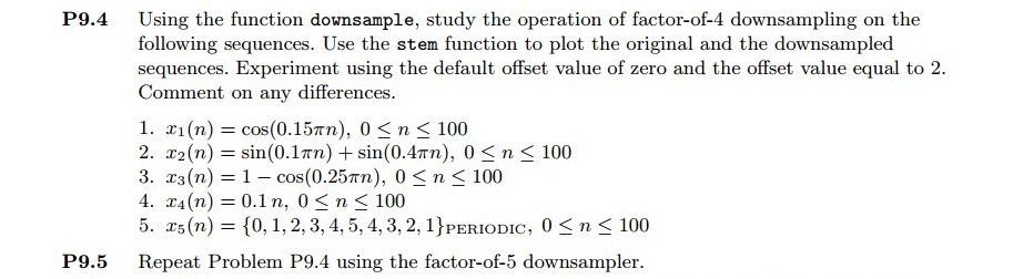
max(magX1)
 
%% --------------------------------------------------------------------
%%              START X(w)'s  mag ang real imag
%% --------------------------------------------------------------------
figure('NumberTitle', 'off', 'Name', 'Problem 9.4.1 X1 DTFT');
set(gcf,'Color','white');
subplot(2,1,1); plot(w/pi,magX1); grid on; %axis([-2, -1, -0.5, 0, 0.15, 0.5, 1, 2]);
title('Magnitude Response');
xlabel('digital frequency in \pi units'); ylabel('Magnitude  |H|');
set(gca, 'xtick', [-2,-1.85,-1.5,-1,-0.15,0,0.15,0.5,1,1.5,1.85,2]);
subplot(2,1,2); plot(w/pi, angX1/pi); grid on;  %axis([-1,1,-1.05,1.05]);
title('Phase Response');
xlabel('digital frequency in \pi units'); ylabel('Radians/\pi');
 
figure('NumberTitle', 'off', 'Name', 'Problem 9.4.1 X1 DTFT');
set(gcf,'Color','white');
subplot(2,1,1); plot(w/pi, realX1); grid on;
title('Real Part');
xlabel('digital frequency in \pi units'); ylabel('Real');
subplot(2,1,2); plot(w/pi, imagX1); grid on;
title('Imaginary Part');
xlabel('digital frequency in \pi units'); ylabel('Imaginary');
%% -------------------------------------------------------------------
%%             END X's  mag ang real imag
%% -------------------------------------------------------------------
 
% ----------------------------
%       DTFT of y
% ----------------------------
M = 500;
[Y, w] = dtft1(y, ny, M);
 
magY_DTFT = abs(Y);  angY_DTFT = angle(Y);  realY_DTFT = real(Y);  imagY_DTFT = imag(Y);
max(magY_DTFT)
ratio = max(magX1)/max(magY_DTFT)
 
%% --------------------------------------------------------------------
%%              START Y(w)'s  mag ang real imag
%% --------------------------------------------------------------------
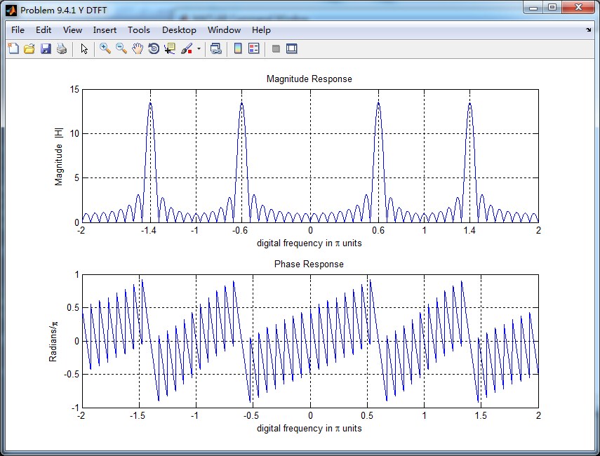
figure('NumberTitle', 'off', 'Name', 'Problem 9.4.1 Y DTFT');
set(gcf,'Color','white');
subplot(2,1,1); plot(w/pi, magY_DTFT); grid on;  %axis([-2,2, -1, 2]);
title('Magnitude Response');
xlabel('digital frequency in \pi units'); ylabel('Magnitude  |H|');
set(gca, 'xtick', [-2,-1.4,-1,-0.6,0,0.6,1,1.4,2]);
subplot(2,1,2); plot(w/pi, angY_DTFT/pi); grid on;  %axis([-1,1,-1.05,1.05]);
title('Phase Response');
xlabel('digital frequency in \pi units'); ylabel('Radians/\pi');
 
figure('NumberTitle', 'off', 'Name', 'Problem 9.4.1 Y DTFT');
set(gcf,'Color','white');
subplot(2,1,1); plot(w/pi, realY_DTFT); grid on;
title('Real Part');
xlabel('digital frequency in \pi units'); ylabel('Real');
subplot(2,1,2); plot(w/pi, imagY_DTFT); grid on;
title('Imaginary Part');
xlabel('digital frequency in \pi units'); ylabel('Imaginary');
%% -------------------------------------------------------------------
%%             END Y's  mag ang real imag
%% -------------------------------------------------------------------
 
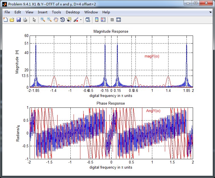
figure('NumberTitle', 'off', 'Name', sprintf('Problem 9.4.1 X1 & Y--DTFT of x and y, D=%d offset=%d', D,OFFSET));
set(gcf,'Color','white');
subplot(2,1,1); plot(w/pi,magX1); grid on;  %axis([-1,1,0,1.05]);
title('Magnitude Response');
xlabel('digital frequency in \pi units'); ylabel('Magnitude  |H|');
set(gca, 'xtick', [-2,-1.85,-1.4,-1,-0.6,-0.5,-0.15,0,0.15,0.5,0.6,1,1.4,1.85,2]);
set(gca, 'ytick', [-0.2, 0, 13.5, 20, 40, 51, 60]);
hold on;
plot(w/pi, magY_DTFT, 'r'); gtext('magY(\omega)', 'Color', 'r');
hold off;
 
subplot(2,1,2); plot(w/pi, angX1/pi); grid on;  %axis([-1,1,-1.05,1.05]);
title('Phase Response');
xlabel('digital frequency in \pi units'); ylabel('Radians/\pi');
hold on;
plot(w/pi, angY_DTFT/pi, 'r'); gtext('AngY(\omega)', 'Color', 'r');
hold off;

　　运行结果：

分两种情况

1、按照D=4抽取，offset=0

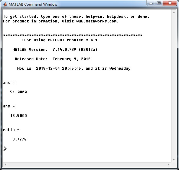
原始序列，抽取序列

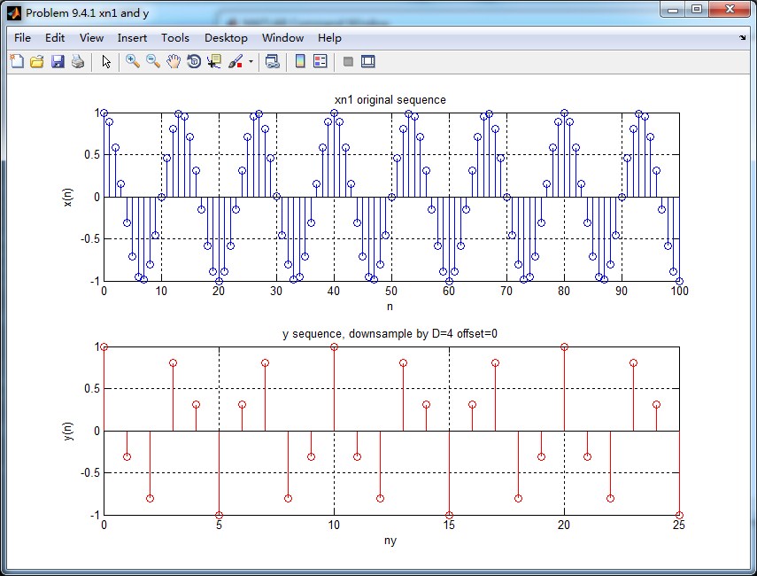
原始序列的谱

抽取序列的谱

二者的DTFT混叠到一起，红颜色曲线是抽取序列的DTFT，可看出，其幅度大致为原始序列的谱幅度的1/4（精确值是1/3.7778）。

2、按照D=4抽取，offset=2

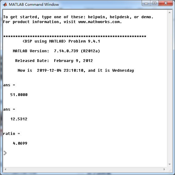
二者的DTFT混叠到一起，红颜色曲线是抽取序列的DTFT，可看出，其幅度大致为原始序列的谱幅度的1/4（精确值是1/4.0699）。