机器学习与Tensorflow（3）—— 机器学习及MNIST数据集分类优化

一、二次代价函数

1. 形式：

其中，C为代价函数，X表示样本，Y表示实际值，a表示输出值，n为样本总数

2. 利用梯度下降法调整权值参数大小，推导过程如下图所示：

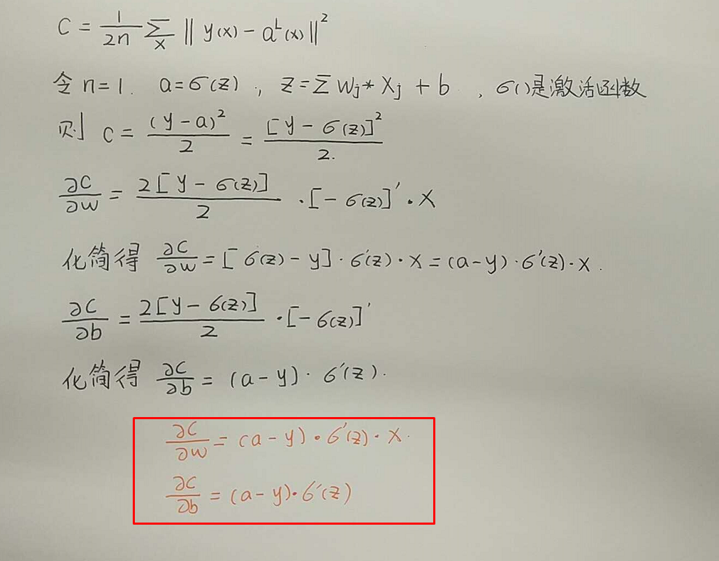
根据结果可得，权重w和偏置b的梯度跟激活函数的梯度成正比（即激活函数的梯度越大，w和b的大小调整的越快，训练速度也越快）

3. 激活函数是sigmoid函数时，二次代价函数调整参数过程分析

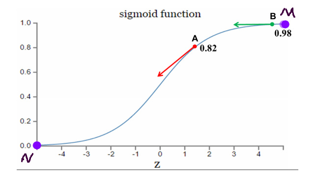
理想调整参数状态：距离目标点远时，梯度大，参数调整较快；距离目标点近时，梯度小，参数调整较慢。
如果我的目标点是调整到M点，从A点==>B点的调整过程，A点距离目标点远，梯度大，调整参数较快；B点距离目标较近，梯度小，调整参数慢。符合参数调整策略
如果我的目标点是调整到N点，从B点==>A点的调整过程，A点距离目标点近，梯度大，调整参数较快；B点距离目标较远，梯度小，调整参数慢。不符合参数调整策略

二、交叉熵代价函数

1.形式：

其中，C为代价函数，X表示样本，Y表示实际值，a表示输出值，n为样本总数

2. 利用梯度下降法调整权值参数大小，推导过程如下图所示：

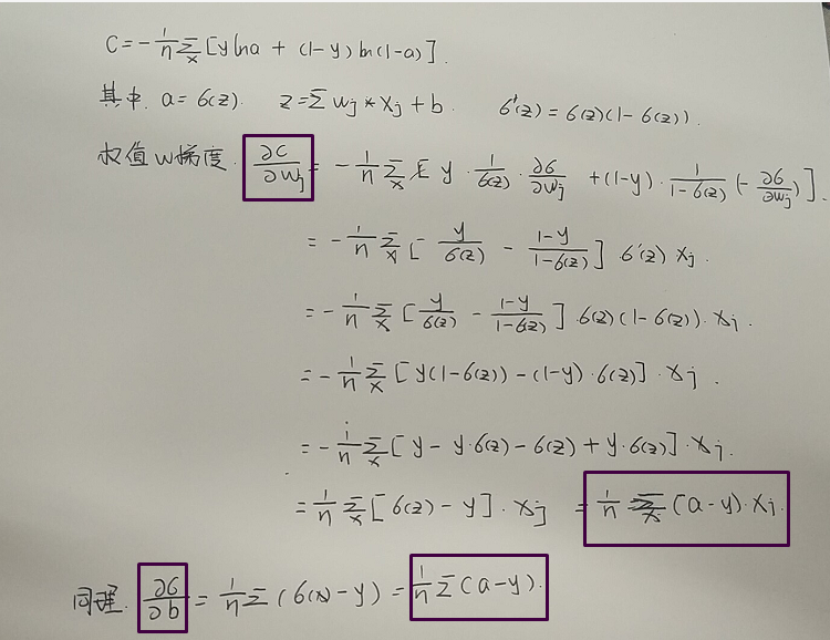
根据结果可得，权重w和偏置b的梯度跟激活函数的梯度无关。而和输出值与实际值的误差成正比（即误差越大，w和b的大小调整的越快，训练速度也越快）

3.激活函数是sigmoid函数时，二次代价函数调整参数过程分析

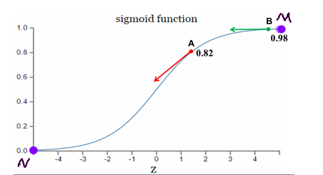
理想调整参数状态：距离目标点远时，梯度大，参数调整较快；距离目标点近时，梯度小，参数调整较慢。
如果我的目标点是调整到M点，从A点==>B点的调整过程，A点距离目标点远，误差大，调整参数较快；B点距离目标较近，误差小，调整参数较慢。符合参数调整策略
如果我的目标点是调整到N点，从B点==>A点的调整过程，A点距离目标点近，误差小，调整参数较慢；B点距离目标较远，误差大，调整参数较快。符合参数调整策略

总结：

• 如果输出神经元是线性的，选择二次代价函数较为合适
• 如果输出神经元是S型函数（sigmoid函数），选择交叉熵代价函数较为合适
• 如果输出神经元是softmax回归的代价函数，选择对数释然代价函数较为合适

二、利用代价函数优化MNIST数据集识别程序

1.在Tensorflow中代价函数的选择：

如果输出神经元是线性的，选择二次代价函数较为合适 loss = tf.reduce_mean(tf.square())
如果输出神经元是S型函数（sigmoid函数），选择交叉熵代价函数较为合适 loss = tf.reduce_mean(tf.nn.sigmoid_cross_entropy_with_logits())
如果输出神经元是softmax回归的代价函数，选择对数释然代价函数较为合适 loss = tf.reduce_mean(tf.nn.softmax_cross_entropy_with_logits())

2.通过代价函数选择对MNIST数据集分类程序优化

#使用交叉熵代价函数

 import os
 os.environ['TF_CPP_MIN_LOG_LEVEL'] = ''
 import tensorflow as tf
 from tensorflow.examples.tutorials.mnist import input_data
 #载入数据集
 mnist = input_data.read_data_sets('MNIST_data', one_hot=True)
 #每个批次的大小（即每次训练的图片数量）
 batch_size = 50
 #计算一共有多少个批次
 n_bitch = mnist.train.num_examples // batch_size
 #定义两个placeholder
 x = tf.placeholder(tf.float32, [None, 784])
 y = tf.placeholder(tf.float32, [None, 10])
 #创建一个只有输入层（784个神经元）和输出层（10个神经元）的简单神经网络
 Weights = tf.Variable(tf.zeros([784, 10]))
 Biases = tf.Variable(tf.zeros([10]))
 Wx_plus_B = tf.matmul(x, Weights) + Biases
 prediction = tf.nn.softmax(Wx_plus_B)
 #交叉熵代价函数
 loss = tf.reduce_mean(tf.nn.softmax_cross_entropy_with_logits(labels=y, logits=prediction))
 #使用梯度下降法
 train_step = tf.train.GradientDescentOptimizer(0.15).minimize(loss)
 #初始化变量
 init = tf.global_variables_initializer()
 #结果存放在一个布尔型列表中
 correct_prediction = tf.equal(tf.argmax(y, 1), tf.argmax(prediction, 1)) #argmax返回一维张量中最大的值所在的位置，标签值和预测值相同，返回为True
 #求准确率
 accuracy = tf.reduce_mean(tf.cast(correct_prediction, tf.float32)) #cast函数将correct_prediction的布尔型转换为浮点型，然后计算平均值即为准确率

 with tf.Session() as sess:
     sess.run(init)
     #将测试集循环训练20次
     for epoch in range(21):
         #将测试集中所有数据循环一次
         for batch in range(n_bitch):
             batch_xs, batch_ys = mnist.train.next_batch(batch_size)   #取测试集中batch_size数量的图片及对应的标签值
             sess.run(train_step, feed_dict={x:batch_xs, y:batch_ys})  #将上一行代码取到的数据进行训练
         acc = sess.run(accuracy, feed_dict={x:mnist.test.images, y:mnist.test.labels})  #准确率的计算
         print('Iter : ' + str(epoch) + ',Testing Accuracy = ' + str(acc))

#执行结果

 Iter : 0,Testing Accuracy = 0.8323
 Iter : 1,Testing Accuracy = 0.8947
 Iter : 2,Testing Accuracy = 0.9032
 Iter : 3,Testing Accuracy = 0.9068
 Iter : 4,Testing Accuracy = 0.909
 Iter : 5,Testing Accuracy = 0.9105
 Iter : 6,Testing Accuracy = 0.9126
 Iter : 7,Testing Accuracy = 0.9131
 Iter : 8,Testing Accuracy = 0.9151
 Iter : 9,Testing Accuracy = 0.9168
 Iter : 10,Testing Accuracy = 0.9178
 Iter : 11,Testing Accuracy = 0.9173
 Iter : 12,Testing Accuracy = 0.9181
 Iter : 13,Testing Accuracy = 0.9194
 Iter : 14,Testing Accuracy = 0.9201
 Iter : 15,Testing Accuracy = 0.9197
 Iter : 16,Testing Accuracy = 0.9213
 Iter : 17,Testing Accuracy = 0.9212
 Iter : 18,Testing Accuracy = 0.9205
 Iter : 19,Testing Accuracy = 0.9215

#使用二次代价函数

 import os
 os.environ['TF_CPP_MIN_LOG_LEVEL'] = ''
 import tensorflow as tf
 from tensorflow.examples.tutorials.mnist import input_data
 #载入数据集
 mnist = input_data.read_data_sets('MNIST_data', one_hot=True)
 #每个批次的大小（即每次训练的图片数量）
 batch_size = 100
 #计算一共有多少个批次
 n_bitch = mnist.train.num_examples // batch_size
 #定义两个placeholder
 x = tf.placeholder(tf.float32, [None, 784])
 y = tf.placeholder(tf.float32, [None, 10])
 #创建一个只有输入层（784个神经元）和输出层（10个神经元）的简单神经网络
 Weights = tf.Variable(tf.zeros([784, 10]))
 Biases = tf.Variable(tf.zeros([10]))
 Wx_plus_B = tf.matmul(x, Weights) + Biases
 prediction = tf.nn.softmax(Wx_plus_B)
 #二次代价函数
 loss = tf.reduce_mean(tf.square(y - prediction))
 #使用梯度下降法
 train_step = tf.train.GradientDescentOptimizer(0.2).minimize(loss)
 #初始化变量
 init = tf.global_variables_initializer()
 #结果存放在一个布尔型列表中
 correct_prediction = tf.equal(tf.argmax(y, 1), tf.argmax(prediction, 1)) #argmax返回一维张量中最大的值所在的位置，标签值和预测值相同，返回为True
 #求准确率
 accuracy = tf.reduce_mean(tf.cast(correct_prediction, tf.float32)) #cast函数将correct_prediction的布尔型转换为浮点型，然后计算平均值即为准确率

 with tf.Session() as sess:
     sess.run(init)
     #将测试集循环训练20次
     for epoch in range(21):
         #将测试集中所有数据循环一次
         for batch in range(n_bitch):
             batch_xs, batch_ys = mnist.train.next_batch(batch_size)   #取测试集中batch_size数量的图片及对应的标签值
             sess.run(train_step, feed_dict={x:batch_xs, y:batch_ys})  #将上一行代码取到的数据进行训练
         acc = sess.run(accuracy, feed_dict={x:mnist.test.images, y:mnist.test.labels})  #准确率的计算
         print('Iter : ' + str(epoch) + ',Testing Accuracy = ' + str(acc))

#执行结果

 Iter : 0,Testing Accuracy = 0.8325
 Iter : 1,Testing Accuracy = 0.8711
 Iter : 2,Testing Accuracy = 0.8831
 Iter : 3,Testing Accuracy = 0.8876
 Iter : 4,Testing Accuracy = 0.8942
 Iter : 5,Testing Accuracy = 0.898
 Iter : 6,Testing Accuracy = 0.9002
 Iter : 7,Testing Accuracy = 0.9014
 Iter : 8,Testing Accuracy = 0.9036
 Iter : 9,Testing Accuracy = 0.9052
 Iter : 10,Testing Accuracy = 0.9065
 Iter : 11,Testing Accuracy = 0.9073
 Iter : 12,Testing Accuracy = 0.9084
 Iter : 13,Testing Accuracy = 0.909
 Iter : 14,Testing Accuracy = 0.9095
 Iter : 15,Testing Accuracy = 0.9115
 Iter : 16,Testing Accuracy = 0.912
 Iter : 17,Testing Accuracy = 0.9126
 Iter : 18,Testing Accuracy = 0.913
 Iter : 19,Testing Accuracy = 0.9136
 Iter : 20,Testing Accuracy = 0.914

结论：（二者只有代价函数不同）

• 正确率达到90%所用迭代次数：使用交叉熵代价函数为第三次；使用二次代价函数为第六次（在MNIST数据集分类中，使用交叉熵代价函数收敛速度较快）
• 最终正确率：使用交叉熵代价函数为92.15%，使用二次代价函数为91.4%（在MNIST数据集分类中，使用交叉熵代价函数识别准确率较高）

三、拟合问题

参考文章：
https://blog.csdn.net/willduan1/article/details/53070777

1.根据拟合结果分类：

• 欠拟合：模型没有很好地捕捉到数据特征，不能够很好地拟合数据
• 正确拟合
• 过拟合：模型把数据学习的太彻底，以至于把噪声数据的特征也学习到了，这样就会导致在后期测试的时候不能够很好地识别数据，即不能正确的分类，模型泛化能力太差

2.解决欠拟合和过拟合

解决欠拟合常用方法：

• 添加其他特征项，有时候我们模型出现欠拟合的时候是因为特征项不够导致的，可以添加其他特征项来很好地解决。
• 添加多项式特征，这个在机器学习算法里面用的很普遍，例如将线性模型通过添加二次项或者三次项使模型泛化能力更强。
• 减少正则化参数，正则化的目的是用来防止过拟合的，但是现在模型出现了欠拟合，则需要减少正则化参数。

解决过拟合常用方法：

• 增加数据集
• 正则化方法
• Dropout（通俗一点讲就是dropout方法在训练的时候让神经元以一定的概率不工作）

四、初始化优化MNIST数据集分类问题

#改变初始化方法

Weights = tf.Variable(tf.truncated_normal([784, 10]))
Biases = tf.Variable(tf.zeros([10]) + 0.1)

五、优化器优化MNIST数据集分类问题

大多数机器学习任务就是最小化损失，在损失定义的情况下，后面的工作就交给优化器。
因为深度学习常见的是对于梯度的优化，也就是说，优化器最后其实就是各种对于梯度下降算法的优化。

1.梯度下降法分类及其介绍

• 标准梯度下降法：先计算所有样本汇总误差，然后根据总误差来更新权值
• 随机梯度下降法：随机抽取一个样本来计算误差，然后更新权值
• 批量梯度下降法：是一种折中方案，从总样本中选取一个批次（batch），然后计算这个batch的总误差，根据总误差来更新权值

2.常见优化器介绍

参考文章：
https://www.leiphone.com/news/201706/e0PuNeEzaXWsMPZX.html

3.优化器优化MNIST数据集分类问题

#选择Adam优化器

 import os
 os.environ['TF_CPP_MIN_LOG_LEVEL'] = ''
 import tensorflow as tf
 from tensorflow.examples.tutorials.mnist import input_data
 #载入数据集
 mnist = input_data.read_data_sets('MNIST_data', one_hot=True)
 #每个批次的大小（即每次训练的图片数量）
 batch_size = 50
 #计算一共有多少个批次
 n_bitch = mnist.train.num_examples // batch_size
 #定义两个placeholder
 x = tf.placeholder(tf.float32, [None, 784])
 y = tf.placeholder(tf.float32, [None, 10])
 #创建一个只有输入层（784个神经元）和输出层（10个神经元）的简单神经网络
 Weights = tf.Variable(tf.zeros([784, 10]))
 Biases = tf.Variable(tf.zeros([10]))
 Wx_plus_B = tf.matmul(x, Weights) + Biases
 prediction = tf.nn.softmax(Wx_plus_B)
 #交叉熵代价函数
 loss = tf.reduce_mean(tf.nn.softmax_cross_entropy_with_logits(labels=y, logits=prediction))
 #使用Adam优化器
 train_step = tf.train.AdamOptimizer(1e-2).minimize(loss)
 #初始化变量
 init = tf.global_variables_initializer()
 #结果存放在一个布尔型列表中
 correct_prediction = tf.equal(tf.argmax(y, 1), tf.argmax(prediction, 1)) #argmax返回一维张量中最大的值所在的位置，标签值和预测值相同，返回为True
 #求准确率
 accuracy = tf.reduce_mean(tf.cast(correct_prediction, tf.float32)) #cast函数将correct_prediction的布尔型转换为浮点型，然后计算平均值即为准确率

 with tf.Session() as sess:
     sess.run(init)
     #将测试集循环训练20次
     for epoch in range(21):
         #将测试集中所有数据循环一次
         for batch in range(n_bitch):
             batch_xs, batch_ys = mnist.train.next_batch(batch_size)   #取测试集中batch_size数量的图片及对应的标签值
             sess.run(train_step, feed_dict={x:batch_xs, y:batch_ys})  #将上一行代码取到的数据进行训练
         acc = sess.run(accuracy, feed_dict={x:mnist.test.images, y:mnist.test.labels})  #准确率的计算
         print('Iter : ' + str(epoch) + ',Testing Accuracy = ' + str(acc))

#执行结果

Iter : 1,Testing Accuracy = 0.9224
Iter : 2,Testing Accuracy = 0.9293
Iter : 3,Testing Accuracy = 0.9195
Iter : 4,Testing Accuracy = 0.9282
Iter : 5,Testing Accuracy = 0.926
Iter : 6,Testing Accuracy = 0.9291
Iter : 7,Testing Accuracy = 0.9288
Iter : 8,Testing Accuracy = 0.9274
Iter : 9,Testing Accuracy = 0.9277
Iter : 10,Testing Accuracy = 0.9249
Iter : 11,Testing Accuracy = 0.9313
Iter : 12,Testing Accuracy = 0.9301
Iter : 13,Testing Accuracy = 0.9315
Iter : 14,Testing Accuracy = 0.9295
Iter : 15,Testing Accuracy = 0.9299
Iter : 16,Testing Accuracy = 0.9303
Iter : 17,Testing Accuracy = 0.93
Iter : 18,Testing Accuracy = 0.9304
Iter : 19,Testing Accuracy = 0.9269
Iter : 20,Testing Accuracy = 0.9273

注意：不同优化器参数的设置是关键。在机器学习中，参数的调整应该是技术加经验，而不是盲目调整。这边是我以后需要学习和积累的地方

六、根据今天所学内容，对MNIST数据集分类进行优化，准确率达到95%以上

#优化程序

 import os
 os.environ['TF_CPP_MIN_LOG_LEVEL'] = ''
 import tensorflow as tf
 from tensorflow.examples.tutorials.mnist import input_data
 #载入数据集
 mnist = input_data.read_data_sets('MNIST_data', one_hot=True)
 #每个批次的大小（即每次训练的图片数量）
 batch_size = 50
 #计算一共有多少个批次
 n_bitch = mnist.train.num_examples // batch_size
 #定义两个placeholder
 x = tf.placeholder(tf.float32, [None, 784])
 y = tf.placeholder(tf.float32, [None, 10])
 #创建一个只有输入层（784个神经元）和输出层（10个神经元）的简单神经网络
 Weights1 = tf.Variable(tf.truncated_normal([784, 200]))
 Biases1 = tf.Variable(tf.zeros([200]) + 0.1)
 Wx_plus_B_L1 = tf.matmul(x, Weights1) + Biases1
 L1 = tf.nn.tanh(Wx_plus_B_L1)

 Weights2 = tf.Variable(tf.truncated_normal([200, 50]))
 Biases2 = tf.Variable(tf.zeros([50]) + 0.1)
 Wx_plus_B_L2 = tf.matmul(L1, Weights2) + Biases2
 L2 = tf.nn.tanh(Wx_plus_B_L2)

 Weights3 = tf.Variable(tf.truncated_normal([50, 10]))
 Biases3 = tf.Variable(tf.zeros([10]) + 0.1)
 Wx_plus_B_L3 = tf.matmul(L2, Weights3) + Biases3
 prediction = tf.nn.softmax(Wx_plus_B_L3)

 #交叉熵代价函数
 loss = tf.reduce_mean(tf.nn.softmax_cross_entropy_with_logits(labels=y, logits=prediction))
 #使用梯度下降法
 train_step = tf.train.AdamOptimizer(2e-3).minimize(loss)
 #初始化变量
 init = tf.global_variables_initializer()
 #结果存放在一个布尔型列表中
 correct_prediction = tf.equal(tf.argmax(y, 1), tf.argmax(prediction, 1))
 #求准确率
 accuracy = tf.reduce_mean(tf.cast(correct_prediction, tf.float32))

 with tf.Session() as sess:
     sess.run(init)
     #将测试集循环训练50次
     for epoch in range(51):
         #将测试集中所有数据循环一次
         for batch in range(n_bitch):
             batch_xs, batch_ys = mnist.train.next_batch(batch_size)   #取测试集中batch_size数量的图片及对应的标签值
             sess.run(train_step, feed_dict={x:batch_xs, y:batch_ys})  #将上一行代码取到的数据进行训练
         test_acc = sess.run(accuracy, feed_dict={x:mnist.test.images, y:mnist.test.labels})  #准确率的计算
         print('Iter : ' + str(epoch) + ',Testing Accuracy = ' + str(test_acc))

#执行结果

 Iter : 0,Testing Accuracy = 0.6914
 Iter : 1,Testing Accuracy = 0.7236
 Iter : 2,Testing Accuracy = 0.8269
 Iter : 3,Testing Accuracy = 0.8885
 Iter : 4,Testing Accuracy = 0.9073
 Iter : 5,Testing Accuracy = 0.9147
 Iter : 6,Testing Accuracy = 0.9125
 Iter : 7,Testing Accuracy = 0.922
 Iter : 8,Testing Accuracy = 0.9287
 Iter : 9,Testing Accuracy = 0.9248
 Iter : 10,Testing Accuracy = 0.9263
 Iter : 11,Testing Accuracy = 0.9328
 Iter : 12,Testing Accuracy = 0.9316
 Iter : 13,Testing Accuracy = 0.9387
 Iter : 14,Testing Accuracy = 0.9374
 Iter : 15,Testing Accuracy = 0.9433
 Iter : 16,Testing Accuracy = 0.9419
 Iter : 17,Testing Accuracy = 0.9379
 Iter : 18,Testing Accuracy = 0.9379
 Iter : 19,Testing Accuracy = 0.9462
 Iter : 20,Testing Accuracy = 0.9437
 Iter : 21,Testing Accuracy = 0.9466
 Iter : 22,Testing Accuracy = 0.9479
 Iter : 23,Testing Accuracy = 0.9498
 Iter : 24,Testing Accuracy = 0.9481
 Iter : 25,Testing Accuracy = 0.9489
 Iter : 26,Testing Accuracy = 0.9496
 Iter : 27,Testing Accuracy = 0.95
 Iter : 28,Testing Accuracy = 0.9508
 Iter : 29,Testing Accuracy = 0.9533
 Iter : 30,Testing Accuracy = 0.9509
 Iter : 31,Testing Accuracy = 0.9516
 Iter : 32,Testing Accuracy = 0.9541
 Iter : 33,Testing Accuracy = 0.9513
 Iter : 34,Testing Accuracy = 0.951
 Iter : 35,Testing Accuracy = 0.9556
 Iter : 36,Testing Accuracy = 0.9527
 Iter : 37,Testing Accuracy = 0.9521
 Iter : 38,Testing Accuracy = 0.9546
 Iter : 39,Testing Accuracy = 0.9544
 Iter : 40,Testing Accuracy = 0.9555
 Iter : 41,Testing Accuracy = 0.9546
 Iter : 42,Testing Accuracy = 0.9553
 Iter : 43,Testing Accuracy = 0.9534
 Iter : 44,Testing Accuracy = 0.9576
 Iter : 45,Testing Accuracy = 0.9535
 Iter : 46,Testing Accuracy = 0.9569
 Iter : 47,Testing Accuracy = 0.9556
 Iter : 48,Testing Accuracy = 0.9568
 Iter : 49,Testing Accuracy = 0.956
 Iter : 50,Testing Accuracy = 0.9557

#写在后面

呀呀呀呀

本来想着先把python学差不多再开始机器学习和这些框架的学习

老师触不及防的任务

给了论文 让我搭一个模型出来

我只能硬着头皮上了

不想用公式编译器了

手写版计算过程  请忽略那丑丑的字儿

加油哦！小伙郭