Matplotlib新手上路(下)

接上篇继续，这次来演示下如何做动画，以及加载图片

一、动画图

import numpy as np
import matplotlib.pyplot as plt
import matplotlib.animation as animation
 
fig, ax = plt.subplots()
 
x = np.arange(0, 2 * np.pi, 0.01)
line, = ax.plot(x, np.sin(x))
 
def init():
    line.set_ydata([np.nan] * len(x))  # Y轴值归0，Mac上加不加这句，都一样
    return line,
 
def animate(i):
    line.set_ydata(np.sin(x + i / 100))  # update the data.
    return line,
 
ani = animation.FuncAnimation(
    # blit在Mac上只能设置False，否则动画有残影
    fig, animate, init_func=init, interval=2, blit=False, save_count=50)
 
init()
 
plt.show()

　　

基本套路是：init()函数中给定图象的初始状态，然后animate()函数中每次对函数图象动态调整一点点，最后用FuncAnimation把它们串起来。

再来看一个官网给的比较好玩的示例：

from numpy import sin, cos
import numpy as np
import matplotlib.pyplot as plt
import scipy.integrate as integrate
import matplotlib.animation as animation
 
G = 9.8  # acceleration due to gravity, in m/s^2
L1 = 1.0  # length of pendulum 1 in m
L2 = 1.0  # length of pendulum 2 in m
M1 = 1.0  # mass of pendulum 1 in kg
M2 = 1.0  # mass of pendulum 2 in kg
 
def derivs(state, t):
    dydx = np.zeros_like(state)
    dydx[0] = state[1]
 
    del_ = state[2] - state[0]
    den1 = (M1 + M2) * L1 - M2 * L1 * cos(del_) * cos(del_)
    dydx[1] = (M2 * L1 * state[1] * state[1] * sin(del_) * cos(del_) +
               M2 * G * sin(state[2]) * cos(del_) +
               M2 * L2 * state[3] * state[3] * sin(del_) -
               (M1 + M2) * G * sin(state[0])) / den1
 
    dydx[2] = state[3]
 
    den2 = (L2 / L1) * den1
    dydx[3] = (-M2 * L2 * state[3] * state[3] * sin(del_) * cos(del_) +
               (M1 + M2) * G * sin(state[0]) * cos(del_) -
               (M1 + M2) * L1 * state[1] * state[1] * sin(del_) -
               (M1 + M2) * G * sin(state[2])) / den2
 
    return dydx
 
# create a time array from 0..100 sampled at 0.05 second steps
dt = 0.05
t = np.arange(0.0, 20, dt)
 
# th1 and th2 are the initial angles (degrees)
# w10 and w20 are the initial angular velocities (degrees per second)
th1 = 120.0
w1 = 0.0
th2 = -10.0
w2 = 0.0
 
# initial state
state = np.radians([th1, w1, th2, w2])
 
# integrate your ODE using scipy.integrate.
y = integrate.odeint(derivs, state, t)
 
x1 = L1 * sin(y[:, 0])
y1 = -L1 * cos(y[:, 0])
 
x2 = L2 * sin(y[:, 2]) + x1
y2 = -L2 * cos(y[:, 2]) + y1
 
fig = plt.figure()
ax = fig.add_subplot(111, autoscale_on=False, xlim=(-2, 2), ylim=(-2, 2))
ax.set_aspect('equal')
ax.grid()
 
line, = ax.plot([], [], 'o-', lw=2)
time_template = 'time = %.1fs'
time_text = ax.text(0.05, 0.9, '', transform=ax.transAxes)
 
def init():
    line.set_data([], [])
    time_text.set_text('')
    return line, time_text
 
def animate(i):
    thisx = [0, x1[i], x2[i]]
    thisy = [0, y1[i], y2[i]]
 
    line.set_data(thisx, thisy)
    time_text.set_text(time_template % (i * dt))
    return line, time_text
 
ani = animation.FuncAnimation(fig, animate, np.arange(1, len(y)),
                              interval=25, blit=False, init_func=init)
 
plt.show()

　　

甚至还可以创建一些艺术气息的动画：

import numpy as np
import matplotlib.pyplot as plt
from matplotlib.animation import FuncAnimation
 
# Fixing random state for reproducibility
np.random.seed(19680801)
 
# Create new Figure and an Axes which fills it.
fig = plt.figure(figsize=(5, 5))
ax = fig.add_axes([0, 0, 1, 1], frameon=False)
ax.set_xlim(0, 1), ax.set_xticks([])
ax.set_ylim(0, 1), ax.set_yticks([])
 
# Create rain data
n_drops = 50
rain_drops = np.zeros(n_drops, dtype=[('position', float, 2),
                                      ('size',     float, 1),
                                      ('growth',   float, 1),
                                      ('color',    float, 4)])
 
# Initialize the raindrops in random positions and with
# random growth rates.
rain_drops['position'] = np.random.uniform(0, 1, (n_drops, 2))
rain_drops['growth'] = np.random.uniform(50, 200, n_drops)
 
# Construct the scatter which we will update during animation
# as the raindrops develop.
scat = ax.scatter(rain_drops['position'][:, 0], rain_drops['position'][:, 1],
                  s=rain_drops['size'], lw=0.3, edgecolors=rain_drops['color'],
                  facecolors='none')
 
def update(frame_number):
    # Get an index which we can use to re-spawn the oldest raindrop.
    current_index = frame_number % n_drops
 
    # Make all colors more transparent as time progresses.
    rain_drops['color'][:, 3] -= 1.0/len(rain_drops)
    rain_drops['color'][:, 3] = np.clip(rain_drops['color'][:, 3], 0, 1)
 
    # Make all circles bigger.
    rain_drops['size'] += rain_drops['growth']
 
    # Pick a new position for oldest rain drop, resetting its size,
    # color and growth factor.
    rain_drops['position'][current_index] = np.random.uniform(0, 1, 2)
    rain_drops['size'][current_index] = 5
    rain_drops['color'][current_index] = (0, 0, 0, 1)
    rain_drops['growth'][current_index] = np.random.uniform(50, 200)
 
    # Update the scatter collection, with the new colors, sizes and positions.
    scat.set_edgecolors(rain_drops['color'])
    scat.set_sizes(rain_drops['size'])
    scat.set_offsets(rain_drops['position'])
 
# Construct the animation, using the update function as the animation director.
animation = FuncAnimation(fig, update, interval=10)
plt.show()

　　

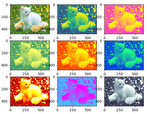
二、加载图片

import matplotlib.pyplot as plt
import matplotlib.image as mpimg
 
img = mpimg.imread('cat.png') # 随便从网上捞的一张图片，保存到当前目录下
lum_img = img[:, :, 0]
 
# plt.figure()
plt.subplot(331)
plt.imshow(img)
 
plt.subplot(332)
plt.imshow(lum_img)
 
plt.subplot(333)
plt.imshow(lum_img, cmap="spring")
 
plt.subplot(334)
plt.imshow(lum_img, cmap="summer")
 
plt.subplot(335)
plt.imshow(lum_img, cmap="autumn")
 
plt.subplot(336)
plt.imshow(lum_img, cmap="winter")
 
plt.subplot(337)
plt.imshow(lum_img, cmap="hot")
 
plt.subplot(338)
plt.imshow(lum_img, cmap="cool")
 
plt.subplot(339)
plt.imshow(lum_img, cmap="bone")
 
plt.show()