利用CNN神经网络实现手写数字mnist分类
题目:
1)In the first step, apply the Convolution Neural Network method to perform the training on one single CPU and testing
2)In the second step, try the distributed training on at least two CPU/GPUs and evaluate the training time.
一、单机单卡实现mnist_CNN
1、CNN的理解
概念:卷积神经网络是一类包含卷积计算且具有深度结构的前馈神经网络,是深度学习代表算法之一。
基本结构:
输入层 —— 【卷积层 —— 激活函数层 —— 池化层 】(隐藏层)—— 全连接层 ——输出层
(1)输入层:原始数据的输入,可对数据进行预处理(如:去均值、归一化)
(2)卷积层:CNN里面最重要的构建单元。
Filter卷积核(相当W): 局部关联,抽取重要特征,是一个类似窗口移动方式的映射窗口,大小可自定义
步长stride: 卷积核移动的大小
填充 Zero-padding :对卷积核边缘填充0,以能计算出相对大小的特征图(feature map), 通常有‘SAME’、‘VALID’ 两个类型
特征图(feature map):经过卷积核对原始图的映射最后得出来的计算结果(数量和同层的卷积核相同)
(3)激活函数层:对卷积层进行非线性变化,有很多种(这里我用的是relu,一般想快点梯度下降的话选这个,简单、收敛快、但较脆弱)
(4)池化层:用于压缩数据和减少参数的量,减小过拟合,也相当于降维
(5)全连接层:神经网络的最后一层,两层之间所有神经元进行全连接
(6)输出层:最后输出结果的层(这里用的是softmax对mnist进行分类)
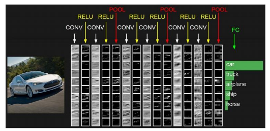
过程类似下图:
2、设计过程
请看图:
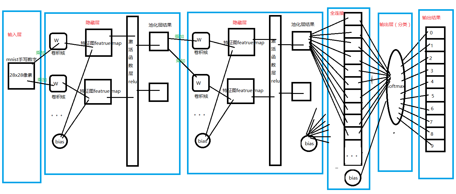
图中画得并不详细,请看代码:
__author__ = 'Kadaj'

import tensorflow as tf
from tensorflow.examples.tutorials.mnist import input_data
import numpy as np

mnist = input_data.read_data_sets('mnist/', one_hot=True)

#创建W , b  构建图
def weight_variable(shape):
    initial = tf.truncated_normal(shape, stddev=0.1)
    return tf.Variable(initial)

def bias_variable(shape):
    initial = tf.constant(0.1, shape=shape)
    return tf.Variable(initial)

#使用TensorFlow中的二维卷积函数
def conv2d(x, W):
    return tf.nn.conv2d(x, W , strides=[1,1,1,1], padding="SAME")

#池化层
def max_pool_2x2(x):
    return tf.nn.max_pool(x, ksize=[1,2,2,1], strides=[1,2,2,1], padding='SAME')

#由于卷积神经网络会利用到空间结构信息,因此需要将一唯的输入向量转为二维的图片结构
x = tf.placeholder(tf.float32, [None, 784])
y_ = tf.placeholder(tf.float32, [None, 10])
x_image = tf.reshape(x, [-1,28,28,1])

W_conv1 = weight_variable([5,5,1,32])
b_conv1 = bias_variable([32])
h_conv1 = tf.nn.relu(conv2d(x_image, W_conv1)+b_conv1)
h_pool1 = max_pool_2x2(h_conv1)

W_conv2 = weight_variable([5,5,32,64])
b_conv2 = bias_variable([64])
h_conv2 = tf.nn.relu(conv2d(h_pool1, W_conv2)+b_conv2)
h_pool2 = max_pool_2x2(h_conv2)

W_fcl = weight_variable([7 * 7 * 64 , 1024])
b_fcl = bias_variable([1024])
h_pool2_flat = tf.reshape(h_pool2, [-1, 7 * 7 * 64 ])
h_fcl = tf.nn.relu(tf.matmul(h_pool2_flat, W_fcl) + b_fcl )

#防止过拟合,使用Dropout层
keep_prob = tf.placeholder(tf.float32)
h_fcl_drop = tf.nn.dropout(h_fcl, keep_prob)

#接着使用softmax分类
W_fc2 = weight_variable([1024,10])
b_fc2 = bias_variable([10])
y_conv = tf.nn.softmax(tf.matmul(h_fcl_drop, W_fc2) + b_fc2)

#定义损失函数
cross_entropy = tf.reduce_mean(-tf.reduce_sum(y_ * tf.log(y_conv), reduction_indices=[1]))
train_step = tf.train.AdamOptimizer(1e-4).minimize(cross_entropy)

#计算正确率
correct_prediction = tf.equal(tf.argmax(y_conv,1) , tf.argmax(y_,1))
accuracy = tf.reduce_mean(tf.cast(correct_prediction, tf.float32))

init = tf.global_variables_initializer()

with tf.Session(config= tf.ConfigProto(log_device_placement = True)) as sess:
    #训练
    sess.run(init)
    for i in range(20001):
        batch = mnist.train.next_batch(50)
        if i % 100 == 0:
            train_accuracy= sess.run( [accuracy ] ,feed_dict={x: batch[0], y_: batch[1], keep_prob: 1.0})
            print("The local_step "+str(i) +" of training accuracy is "+ str(train_accuracy))
        training, cost = sess.run( [train_step,cross_entropy] , feed_dict={x: batch[0], y_: batch[1], keep_prob: 0.5})

    accuracyResult = list(range(10))
    for i in range(10):
        batch = mnist.test.next_batch(1000)
        accuracyResult[i] = sess.run([accuracy], feed_dict={x: batch[0], y_: batch[1], keep_prob: 1.0})
    print("The testing accuracy is :", np.mean(accuracyResult))
    print("The cost function is ", cost)
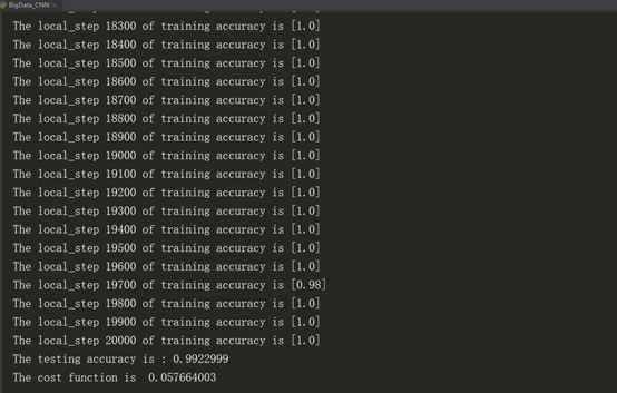
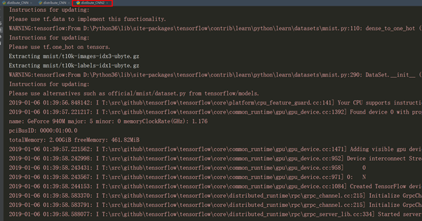
3、执行结果
4、对上述代码的 Dropout补充

在深度学习中,Dropout是最流行的正则化技术,它被证明非常成功,即使在顶尖水准的神经网络中也可以带来1%到2%的准确度提升,这可能听起来不是很多,但是如果模型已经有95%的准确率,获得2%的准确率提升意味着降低错误率40%,即从5%的错误率降低到3%错误率。
在每一次训练step中,每个神经元,包括输入神经元,但是不包括输出神经元,有一个概率被临时丢掉,意味着它将被忽视在整个这次训练step中,但是有可能下次再被激活。
超参数dropout rate,一般设置为50%,在训练之后,神经元不会被dropout 。
二、分布式实现
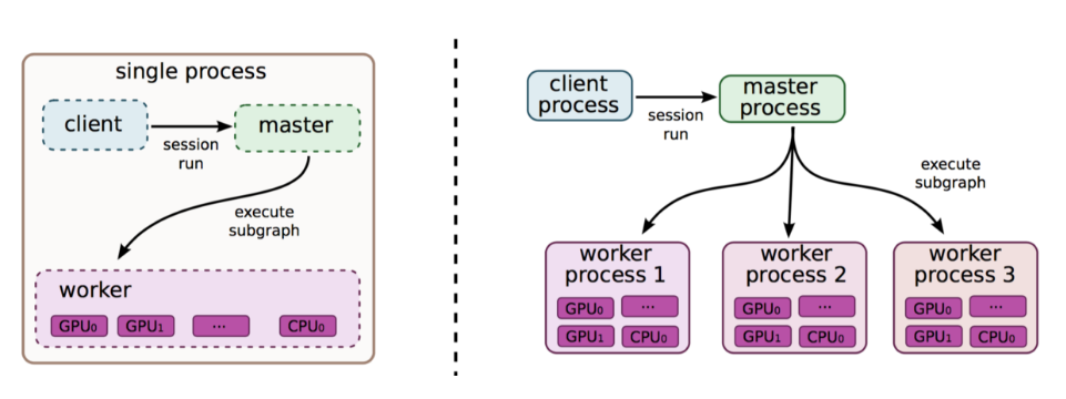
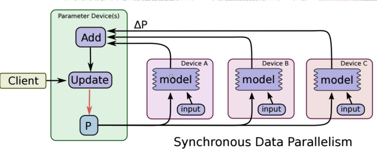
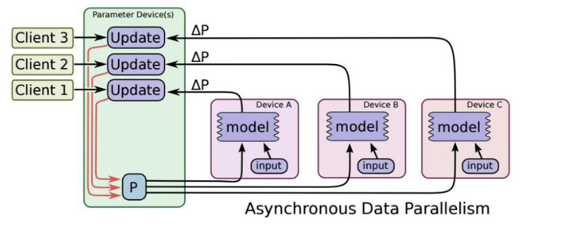
1、分布式原理(此图是单机多卡和多机多卡)
2、基本概念
Cluster、Job、task概念:三者可以简单的看成是层次关系,task可以看成每台机器上的一个进程,多个task组成job,job又有:ps、worker两种,分别用于参数服务、计算服务,组成cluster。
3、同步SGD与异步SGD
同步SGD:各个用于并行计算的电脑,计算完各自的batch后,求取梯度值,把梯度值统一送到ps服务机器中,由ps服务机器求取梯度平均值,更新ps服务器上的参数。
异步SGD:ps服务器只要收到一台机器的梯度值,就直接进行参数更新,无需等待其他机器。这种迭代方法比较不稳定,收敛曲线震动比较厉害,因为当A机器计算完更新了ps中的参数,可能B机器还是在用上一次迭代的旧版参数值。
以上这些来自:https://blog.csdn.net/panpan_1210/aarticle/details/79402105#
4、基本设计
逻辑基本上和第一问是一样的,由于没有找到足够的环境,所以这里利用本机模拟实现分布式训练。
这里直接上代码吧:
import tensorflow as tf
from tensorflow.examples.tutorials.mnist import input_data
import numpy as np

mnist = input_data.read_data_sets('mnist/', one_hot=True)

#创建W , b  构建图
def weight_variable(shape):
    initial = tf.truncated_normal(shape, stddev=0.1)
    return tf.Variable(initial)

def bias_variable(shape):
    initial = tf.constant(0.1, shape=shape)
    return tf.Variable(initial)

#使用TensorFlow中的二维卷积函数
def conv2d(x, W):
    return tf.nn.conv2d(x, W , strides=[1,1,1,1], padding="SAME")

#池化层
def max_pool_2x2(x):
    return tf.nn.max_pool(x, ksize=[1,2,2,1], strides=[1,2,2,1], padding='SAME')

cluster = tf.train.ClusterSpec({
    "worker": [
        "127.0.0.1:23236",
        "127.0.0.1:23237",
    ],
    "ps": [
        "127.0.0.1:32216"
    ]})

isps = False
if isps:
    server = tf.train.Server(cluster, job_name='ps', task_index=0)
    server.join()
else:
    server = tf.train.Server(cluster, job_name='worker', task_index=0)
    with tf.device(tf.train.replica_device_setter(worker_device='/job:worker/task:0/cpu:0', cluster=cluster)):
        # 由于卷积神经网络会利用到空间结构信息,因此需要将一唯的输入向量转为二维的图片结构
        global_step = tf.Variable(0, name='global_step', trainable=False)
        x = tf.placeholder(tf.float32, [None, 784])
        y_ = tf.placeholder(tf.float32, [None, 10])
        x_image = tf.reshape(x, [-1, 28, 28, 1])

        W_conv1 = weight_variable([5, 5, 1, 32])
        b_conv1 = bias_variable([32])
        h_conv1 = tf.nn.relu(conv2d(x_image, W_conv1) + b_conv1)
        h_pool1 = max_pool_2x2(h_conv1)

        W_conv2 = weight_variable([5, 5, 32, 64])
        b_conv2 = bias_variable([64])
        h_conv2 = tf.nn.relu(conv2d(h_pool1, W_conv2) + b_conv2)
        h_pool2 = max_pool_2x2(h_conv2)

        W_fcl = weight_variable([7 * 7 * 64, 1024])
        b_fcl = bias_variable([1024])
        h_pool2_flat = tf.reshape(h_pool2, [-1, 7 * 7 * 64])
        h_fcl = tf.nn.relu(tf.matmul(h_pool2_flat, W_fcl) + b_fcl)

        # 防止过拟合,使用Dropout层
        keep_prob = tf.placeholder(tf.float32)
        h_fcl_drop = tf.nn.dropout(h_fcl, keep_prob)

        # 接着使用softmax分类
        W_fc2 = weight_variable([1024, 10])
        b_fc2 = bias_variable([10])
        y_conv = tf.nn.softmax(tf.matmul(h_fcl_drop, W_fc2) + b_fc2)

        #定义损失函数
        cross_entropy = tf.reduce_mean(-tf.reduce_sum(y_ * tf.log(y_conv), reduction_indices=[1]))
        train_step = tf.train.AdamOptimizer(1e-4).minimize(cross_entropy,global_step=global_step)

        correct_prediction = tf.equal(tf.argmax(y_conv,1) , tf.argmax(y_,1))
        accuracy = tf.reduce_mean(tf.cast(correct_prediction, tf.float32))

saver = tf.train.Saver()
summary_op = tf.summary.merge_all()

init_op = tf.initialize_all_variables()
sv = tf.train.Supervisor(init_op=init_op, summary_op=summary_op, saver=saver,global_step=global_step)

config = tf.ConfigProto()
config.gpu_options.allow_growth = True
sum = 0
with sv.managed_session(server.target,config=config) as sess:
    for i in range(10001):
        batch = mnist.train.next_batch(50)
        if i % 100 == 0:
            train_accuracy,step, cost = sess.run( [accuracy ,global_step,cross_entropy] ,feed_dict={x: batch[0], y_: batch[1], keep_prob: 1.0})
            print("The local_step "+str(i) +" of training accuracy is "+ str(train_accuracy)+" and global_step is "+str(step))
        training, cost = sess.run([train_step, cross_entropy],feed_dict={x: batch[0], y_: batch[1], keep_prob: 0.5})
        # sum +=cost

    accuracyResult = list(range(10))
    for i in range(10):
        batch = mnist.test.next_batch(1000)
        accuracyResult[i] = sess.run([accuracy], feed_dict={x: batch[0], y_: batch[1], keep_prob: 1.0})
    print("Test accuracy is :", np.mean(accuracyResult))
    print("The cost function is ", cost)
import tensorflow as tf
from tensorflow.examples.tutorials.mnist import input_data
import numpy as np

mnist = input_data.read_data_sets('mnist/', one_hot=True)

#创建W , b  构建图
def weight_variable(shape):
    initial = tf.truncated_normal(shape, stddev=0.1)
    return tf.Variable(initial)

def bias_variable(shape):
    initial = tf.constant(0.1, shape=shape)
    return tf.Variable(initial)

#使用TensorFlow中的二维卷积函数
def conv2d(x, W):
    return tf.nn.conv2d(x, W , strides=[1,1,1,1], padding="SAME")

#池化层
def max_pool_2x2(x):
    return tf.nn.max_pool(x, ksize=[1,2,2,1], strides=[1,2,2,1], padding='SAME')

cluster = tf.train.ClusterSpec({
    "worker": [
        "127.0.0.1:23236",
        "127.0.0.1:23237",
    ],
    "ps": [
        "127.0.0.1:32216"
    ]})

isps = False
if isps:
    server = tf.train.Server(cluster, job_name='ps', task_index=0)
    server.join()
else:
    server = tf.train.Server(cluster, job_name='worker', task_index=1)
    with tf.device(tf.train.replica_device_setter(worker_device='/job:worker/task:1/cpu:0', cluster=cluster)):
        # 由于卷积神经网络会利用到空间结构信息,因此需要将一唯的输入向量转为二维的图片结构
        global_step = tf.Variable(0, name='global_step', trainable=False)
        x = tf.placeholder(tf.float32, [None, 784])
        y_ = tf.placeholder(tf.float32, [None, 10])
        x_image = tf.reshape(x, [-1, 28, 28, 1])

        W_conv1 = weight_variable([5, 5, 1, 32])
        b_conv1 = bias_variable([32])
        h_conv1 = tf.nn.relu(conv2d(x_image, W_conv1) + b_conv1)
        h_pool1 = max_pool_2x2(h_conv1)

        W_conv2 = weight_variable([5, 5, 32, 64])
        b_conv2 = bias_variable([64])
        h_conv2 = tf.nn.relu(conv2d(h_pool1, W_conv2) + b_conv2)
        h_pool2 = max_pool_2x2(h_conv2)

        W_fcl = weight_variable([7 * 7 * 64, 1024])
        b_fcl = bias_variable([1024])
        h_pool2_flat = tf.reshape(h_pool2, [-1, 7 * 7 * 64])
        h_fcl = tf.nn.relu(tf.matmul(h_pool2_flat, W_fcl) + b_fcl)

        # 防止过拟合,使用Dropout层
        keep_prob = tf.placeholder(tf.float32)
        h_fcl_drop = tf.nn.dropout(h_fcl, keep_prob)

        # 接着使用softmax分类
        W_fc2 = weight_variable([1024, 10])
        b_fc2 = bias_variable([10])
        y_conv = tf.nn.softmax(tf.matmul(h_fcl_drop, W_fc2) + b_fc2)

        #定义损失函数
        cross_entropy = tf.reduce_mean(-tf.reduce_sum(y_ * tf.log(y_conv), reduction_indices=[1]))
        train_step = tf.train.AdamOptimizer(1e-4).minimize(cross_entropy,global_step=global_step)

        correct_prediction = tf.equal(tf.argmax(y_conv,1) , tf.argmax(y_,1))
        accuracy = tf.reduce_mean(tf.cast(correct_prediction, tf.float32))

saver = tf.train.Saver()
summary_op = tf.summary.merge_all()

init_op = tf.initialize_all_variables()
sv = tf.train.Supervisor(init_op=init_op, summary_op=summary_op, saver=saver,global_step=global_step)

config = tf.ConfigProto()
config.gpu_options.allow_growth = True
sum =0
with sv.managed_session(server.target,config=config) as sess:
    for i in range(10001):
        batch = mnist.train.next_batch(50)
        if i % 100 == 0:
            train_accuracy,step = sess.run( [accuracy ,global_step] ,feed_dict={x: batch[0], y_: batch[1], keep_prob: 1.0})
            print("The local_step "+str(i) +" of training accuracy is "+ str(train_accuracy)+" and global_step is "+str(step))
        training, cost = sess.run([train_step, cross_entropy],feed_dict={x: batch[0], y_: batch[1], keep_prob: 0.5})
        # sum +=cost

    accuracyResult = list(range(10))
    for i in range(10):
        batch = mnist.test.next_batch(1000)
        accuracyResult[i] = sess.run([accuracy], feed_dict={x: batch[0], y_: batch[1], keep_prob: 1.0})
    print("Test accuracy is :", np.mean(accuracyResult))
    print("The cost function is ", cost)
import tensorflow as tf
from tensorflow.examples.tutorials.mnist import input_data
import numpy as np

mnist = input_data.read_data_sets('mnist/', one_hot=True)

#创建W , b  构建图
def weight_variable(shape):
    initial = tf.truncated_normal(shape, stddev=0.1)
    return tf.Variable(initial)

def bias_variable(shape):
    initial = tf.constant(0.1, shape=shape)
    return tf.Variable(initial)

#使用TensorFlow中的二维卷积函数
def conv2d(x, W):
    return tf.nn.conv2d(x, W , strides=[1,1,1,1], padding="SAME")

#池化层
def max_pool_2x2(x):
    return tf.nn.max_pool(x, ksize=[1,2,2,1], strides=[1,2,2,1], padding='SAME')

cluster = tf.train.ClusterSpec({
    "worker": [
        "127.0.0.1:23236",
        "127.0.0.1:23237",
    ],
    "ps": [
        "127.0.0.1:32216"
    ]})

isps = True
if isps:
    server = tf.train.Server(cluster, job_name='ps', task_index=0)
    server.join()
else:
    server = tf.train.Server(cluster, job_name='worker', task_index=0)
    with tf.device(tf.train.replica_device_setter(worker_device='/job:worker/task:0/cpu:0', cluster=cluster)):
        # 由于卷积神经网络会利用到空间结构信息,因此需要将一唯的输入向量转为二维的图片结构
        global_step = tf.Variable(0, name='global_step', trainable=False)
        x = tf.placeholder(tf.float32, [None, 784])
        y_ = tf.placeholder(tf.float32, [None, 10])
        x_image = tf.reshape(x, [-1, 28, 28, 1])

        W_conv1 = weight_variable([5, 5, 1, 32])
        b_conv1 = bias_variable([32])
        h_conv1 = tf.nn.relu(conv2d(x_image, W_conv1) + b_conv1)
        h_pool1 = max_pool_2x2(h_conv1)

        W_conv2 = weight_variable([5, 5, 32, 64])
        b_conv2 = bias_variable([64])
        h_conv2 = tf.nn.relu(conv2d(h_pool1, W_conv2) + b_conv2)
        h_pool2 = max_pool_2x2(h_conv2)

        W_fcl = weight_variable([7 * 7 * 64, 1024])
        b_fcl = bias_variable([1024])
        h_pool2_flat = tf.reshape(h_pool2, [-1, 7 * 7 * 64])
        h_fcl = tf.nn.relu(tf.matmul(h_pool2_flat, W_fcl) + b_fcl)

        # 防止过拟合,使用Dropout层
        keep_prob = tf.placeholder(tf.float32)
        h_fcl_drop = tf.nn.dropout(h_fcl, keep_prob)

        # 接着使用softmax分类
        W_fc2 = weight_variable([1024, 10])
        b_fc2 = bias_variable([10])
        y_conv = tf.nn.softmax(tf.matmul(h_fcl_drop, W_fc2) + b_fc2)

        #定义损失函数
        cross_entropy = tf.reduce_mean(-tf.reduce_sum(y_ * tf.log(y_conv), reduction_indices=[1]))
        train_step = tf.train.AdamOptimizer(1e-4).minimize(cross_entropy,global_step=global_step)

        correct_prediction = tf.equal(tf.argmax(y_conv,1) , tf.argmax(y_,1))
        accuracy = tf.reduce_mean(tf.cast(correct_prediction, tf.float32))

saver = tf.train.Saver()
summary_op = tf.summary.merge_all()

init_op = tf.initialize_all_variables()
sv = tf.train.Supervisor(init_op=init_op, summary_op=summary_op, saver=saver,global_step=global_step)

config = tf.ConfigProto()
config.gpu_options.allow_growth = True
sum = 0
with sv.managed_session(server.target,config=config) as sess:
    for i in range(10001):
        batch = mnist.train.next_batch(50)
        if i % 100 == 0:
            train_accuracy,step = sess.run( [accuracy ,global_step] ,feed_dict={x: batch[0], y_: batch[1], keep_prob: 1.0})
            print("The local_step "+str(i) +" of training accuracy is "+ str(train_accuracy)+" and global_step is "+str(step))
        training, cost = sess.run([train_step, cross_entropy],feed_dict={x: batch[0], y_: batch[1], keep_prob: 0.5})
        # sum += cost

    accuracyResult = list(range(10))
    for i in range(10):
        batch = mnist.test.next_batch(1000)
        accuracyResult[i] = sess.run([accuracy], feed_dict={x: batch[0], y_: batch[1], keep_prob: 1.0})
    print("Test accuracy is :", np.mean(accuracyResult))
    print("The cost function is ", cost)
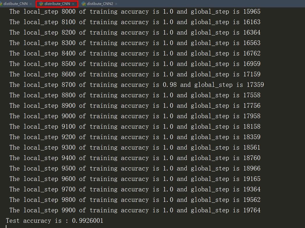
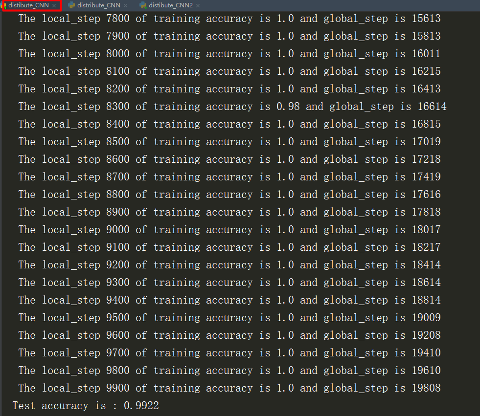
这里模拟了一个ps,两个worker,但是这里训练的时间没有去计算。但是已经迭代减半为10000次
对比了一下单机训练的10000次迭代,正确率只有99.002%
5、执行结果
利用CNN神经网络实现手写数字mnist分类的更多相关文章
- 基于卷积神经网络的手写数字识别分类(Tensorflow)
import numpy as np import tensorflow as tf from tensorflow.examples.tutorials.mnist import input_dat ...
- 利用c++编写bp神经网络实现手写数字识别详解
利用c++编写bp神经网络实现手写数字识别 写在前面 从大一入学开始,本菜菜就一直想学习一下神经网络算法,但由于时间和资源所限,一直未展开比较透彻的学习.大二下人工智能课的修习,给了我一个学习的契机. ...
- 用BP人工神经网络识别手写数字
http://wenku.baidu.com/link?url=HQ-5tZCXBQ3uwPZQECHkMCtursKIpglboBHq416N-q2WZupkNNH3Gv4vtEHyPULezDb5 ...
- TensorFlow卷积神经网络实现手写数字识别以及可视化
边学习边笔记 https://www.cnblogs.com/felixwang2/p/9190602.html # https://www.cnblogs.com/felixwang2/p/9190 ...
- BP神经网络的手写数字识别
BP神经网络的手写数字识别 ANN 人工神经网络算法在实践中往往给人难以琢磨的印象,有句老话叫“出来混总是要还的”,大概是由于具有很强的非线性模拟和处理能力,因此作为代价上帝让它“黑盒”化了.作为一种 ...
- 用Keras搭建神经网络 简单模版(三)—— CNN 卷积神经网络(手写数字图片识别)
# -*- coding: utf-8 -*- import numpy as np np.random.seed(1337) #for reproducibility再现性 from keras.d ...
- TensorFlow.NET机器学习入门【5】采用神经网络实现手写数字识别(MNIST)
从这篇文章开始,终于要干点正儿八经的工作了,前面都是准备工作.这次我们要解决机器学习的经典问题,MNIST手写数字识别. 首先介绍一下数据集.请首先解压:TF_Net\Asset\mnist_png. ...
- keras和tensorflow搭建DNN、CNN、RNN手写数字识别
MNIST手写数字集 MNIST是一个由美国由美国邮政系统开发的手写数字识别数据集.手写内容是0~9,一共有60000个图片样本,我们可以到MNIST官网免费下载,总共4个.gz后缀的压缩文件,该文件 ...
- PyTorch基础——使用卷积神经网络识别手写数字
一.介绍 实验内容 内容包括用 PyTorch 来实现一个卷积神经网络,从而实现手写数字识别任务. 除此之外,还对卷积神经网络的卷积核.特征图等进行了分析,引出了过滤器的概念,并简单示了卷积神经网络的 ...
随机推荐
- python中用psutil模块,yagmail模块监控CPU、硬盘、内存使用,阈值后发送邮件
import yagmailimport psutildef sendmail(subject,contents): #连接邮箱服务器 yag = yagmail.SMTP(user='邮箱名称@16 ...
- Java NIO 入门
本文主要记录 Java 中 NIO 相关的基础知识点,以及基本的使用方式. 一.回顾传统的 I/O 刚接触 Java 中的 I/O 时,使用的传统的 BIO 的 API.由于 BIO 设计的类实在太 ...
- border边框属性
边框属性: 边框宽度(border-width):thin.medium.thick.长度值 边框颜色(border-color):颜色.transparent(透明) 边框样式(border-sty ...
- 常用的phpdoc标签
标签 说明 @access public|private|protected 描述了访问级别.当使用反射技术时,这个标签不是很有用,这是因为API能够自动获取这一特性.在PHPDoc中,用它可略去私有 ...
- UVa 712
这个题根本不用建树,因为是完全二叉树,可以把这个想成二进制.对于根是二进制数的首位,之后依次类推.到最后的叶子节点就是从0到pow(2,n)-1. 关键在于在第一次输入的不是按照x1,x2,x3,x4 ...
- vue修改框架样式/deep/
/deep/ 父元素的样式名 /deep/ 要修改的样式名 使用 ... 貌似不行
- 在Windows下通过压缩包方式安装MySQL
需求:下载MySQL有两种方法,一是下载可执行文件,通过点点点的方式,比较简单没什么技术含量,但是之前通过此方法下载的MySQL与Python进行连接交互的时候总是报1045错误,一直没找到原因,尝试 ...
- [Java Web学习]JDBC事务处理
1. Spring中加入数据库的bean <bean id="dataSource" class="org.apache.commons.dbcp.BasicDat ...
- vue列表拖拽组件 vue-dragging
安装 $ npm install awe-dnd --save 应用 在main.js中,通过Vue.use导入插件 import VueDND from 'awe-dnd' Vue.use(VueD ...
- Educational Codeforces Round 54 (Rated for Div. 2) D:Edge Deletion
题目链接:http://codeforces.com/contest/1076/problem/D 题意:给一个n个点,m条边的无向图.要求保留最多k条边,使得其他点到1点的最短路剩余最多. 思路:当 ...