Deep Learning 5_深度学习UFLDL教程：PCA and Whitening_Exercise（斯坦福大学深度学习教程）

前言

本文是基于Exercise:PCA and Whitening的练习。

理论知识见：UFLDL教程。

实验内容：从10张512*512自然图像中随机选取10000个12*12的图像块（patch），然后对这些patch进行99%的方差保留的PCA计算，最后对这些patch做PCA Whitening和ZCA Whitening，并进行比较。

实验步骤及结果

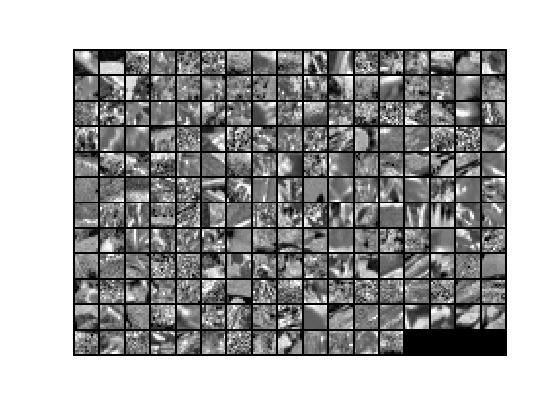
1.加载图像数据，得到10000个图像块为原始数据x，它是144*10000的矩阵，随机显示200个图像块，其结果如下：

2.把它的每个图像块0均值归一化。

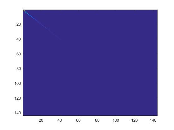
3.PCA降维过程的第一步：求归一化后的原始数据x的协方差矩阵sigma，然后用svd对sigma求出它的U，即原始数据的特征向量或基，再把x投影或旋转到基的方向上，得到新数据xRot。

4.检查PCA实现的第一步是否正确：只需要把xRot的协方差矩阵显示出来。如果是正确的，就会显示出一条直线对角穿过蓝色背景的图片。结果如下：

5.根据要保留99%方差的要求计算出要保留的主成份个数k。

6.PCA降维过程的第二步：保留xRot的前k个成份，后面的全置为0，得到数据xTilde，基U乘以数据xTilde的前k个成份（即：前k行）就得降维后数据xHat。xHat显示结果如下：

为了对比，有0均值归一化后未降维前的数据显示如下：

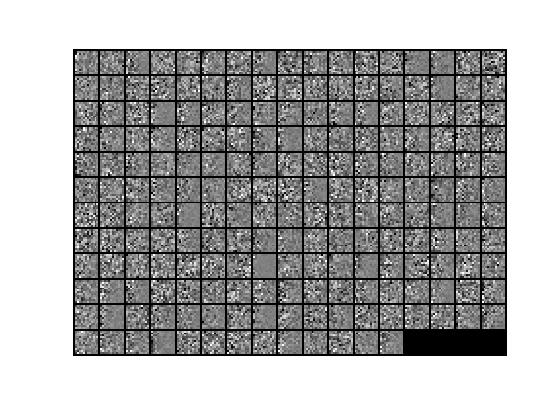
7.对0均值归一化后的数据x实现PCA Whitening，得到PCA白化后的数据xPCAWhite，其显示结果如下：

8.检查PCA白化是否规整化：显示数据xPCAWhite的协方差矩阵。如未规整化，则数据xPCAWhite的协方差矩阵是一个恒等矩阵；如已规整化，则数据xPCAWhite的协方差矩阵的对角线上的值接近于1且依次变小。所以，如未规整化，把epsilon置为0或接近于0，就会得到一条红线对角穿过蓝色背景图片；如已规整化，就会得到就会得到一条从红色渐变到蓝色的线对角穿过蓝色背景的图片。显示结果如下：

9.在PCA Whitening的基础上实现ZCAWhitening，得到的数据xZCAWhite＝U* xPCAWhite。因为前面已经检查过PCA白化，而zca白化是在pca的基础上做的，故这一步不需要再检查。ZCA白化的结果显示如下：

对比PCA白化结果，可以看出，ZCA白化更接近原始数据。

与其相对应的归一化原始数据显示如下：

代码

pca_gen.m

close all;
% clear all;
%%================================================================
%% Step 0a: Load data
% Here we provide the code to load natural image data into x.
% x will be a  *  matrix, where the kth column x(:, k) corresponds to
% the raw image data from the kth 12x12 image patch sampled.
% You do not need to change the code below.

x = sampleIMAGESRAW();
figure('name','Raw images');
randsel = randi(size(x,),,); % A random selection of samples for visualization
display_network(x(:,randsel));

%%================================================================
%% Step 0b: Zero-mean the data (by row)
% You can make use of the mean and repmat/bsxfun functions.

% -------------------- YOUR CODE HERE --------------------
avg = mean(x, );                 %x的每一列的均值
x = x - repmat(avg, size(x, ), );
%%================================================================
%% Step 1a: Implement PCA to obtain xRot
% Implement PCA to obtain xRot, the matrix in which the data is expressed
% with respect to the eigenbasis of sigma, which is the matrix U.

% -------------------- YOUR CODE HERE --------------------
xRot = zeros(size(x)); % You need to compute this
sigma = x * x' / size(x, 2);
[U,S,V]=svd(sigma);
xRot=U'*x;

%%================================================================
%% Step 1b: Check your implementation of PCA
% The covariance matrix for the data expressed with respect to the basis U
% should be a diagonal matrix with non-zero entries only along the main
% diagonal. We will verify this here.
% Write code to compute the covariance matrix, covar.
% When visualised as an image, you should see a straight line across the
% diagonal (non-zero entries) against a blue background (zero entries).

% -------------------- YOUR CODE HERE --------------------
covar = zeros(size(x, )); % You need to compute this
covar = xRot * xRot' / size(xRot, 2);
% Visualise the covariance matrix. You should see a line across the
% diagonal against a blue background.
figure('name','Visualisation of covariance matrix');
imagesc(covar);

%%================================================================
%% Step : Find k, the number of components to retain
% Write code to determine k, the number of components to retain in order
% to retain at least % of the variance.

% -------------------- YOUR CODE HERE --------------------
k = ; % Set k accordingly
sum_k=;
sum=trace(S);
for k=:size(S,)
        sum_k=sum_k+S(k,k);
        if(sum_k/sum>=0.99) %0.9
               break;
       end
end

%%================================================================
%% Step : Implement PCA with dimension reduction
% Now that you have found k, you can reduce the dimension of the data by
% discarding the remaining dimensions. In this way, you can represent the
% data in k dimensions instead of the original , which will save you
% computational time when running learning algorithms on the reduced
% representation.
%
% Following the dimension reduction, invert the PCA transformation to produce
% the matrix xHat, the dimension-reduced data with respect to the original basis.
% Visualise the data and compare it to the raw data. You will observe that
% there is little loss due to throwing away the principal components that
% correspond to dimensions with low variation.

% -------------------- YOUR CODE HERE --------------------
xHat = zeros(size(x));% You need to compute this
xTilde = U(:,:k)' * x;
xHat(:k,:)=xTilde;
xHat=U*xHat;

% Visualise the data, and compare it to the raw data
% You should observe that the raw and processed data are of comparable quality.
% For comparison, you may wish to generate a PCA reduced image which
% retains only % of the variance.

figure('name',['PCA processed images ',sprintf('(%d / %d dimensions)', k, size(x, )),'']);
display_network(xHat(:,randsel));
figure('name','Raw images');
display_network(x(:,randsel));

%%================================================================
%% Step 4a: Implement PCA with whitening and regularisation
% Implement PCA with whitening and regularisation to produce the matrix
% xPCAWhite.

epsilon = 0.1;
xPCAWhite = zeros(size(x));

% -------------------- YOUR CODE HERE --------------------
xPCAWhite = diag(./sqrt(diag(S) + epsilon)) * U' * x;

figure('name','PCA whitened images');
display_network(xPCAWhite(:,randsel));

%%================================================================
%% Step 4b: Check your implementation of PCA whitening
% 检查PCA白化是否规整化。如未规整化，则协方差矩阵是一个恒等矩阵；如已规整化，则其协方差矩阵的对角线上的值接近于1且依次变小。
% Check your implementation of PCA whitening with and without regularisation.
% PCA whitening without regularisation results a covariance matrix
% that is equal to the identity matrix. PCA whitening with regularisation
% results in a covariance matrix with diagonal entries starting close to
%  and gradually becoming smaller. We will verify these properties here.
% Write code to compute the covariance matrix, covar.
%
% 如未规整化，把epsilon置为0或接近于0，就会得到一条红线对角穿过蓝色背景图片。
% 如已规整化，就会得到就会得到一条从红色渐变到蓝色的线对角穿过蓝色背景的图片。
% Without regularisation (set epsilon to  or close to ),
% when visualised as an image, you should see a red line across the
% diagonal (one entries) against a blue background (zero entries).
% With regularisation, you should see a red line that slowly turns
% blue across the diagonal, corresponding to the one entries slowly
% becoming smaller.

% -------------------- YOUR CODE HERE --------------------
covar = zeros(size(xPCAWhite, ));
covar = xPCAWhite * xPCAWhite' / size(xPCAWhite, 2);
% Visualise the covariance matrix. You should see a red line across the
% diagonal against a blue background.
figure('name','Visualisation of covariance matrix');
imagesc(covar);

%%================================================================
%% Step : Implement ZCA whitening
% Now implement ZCA whitening to produce the matrix xZCAWhite.
% Visualise the data and compare it to the raw data. You should observe
% that whitening results in, among other things, enhanced edges.

xZCAWhite = zeros(size(x));

% -------------------- YOUR CODE HERE --------------------
xZCAWhite=U * diag(./sqrt(diag(S) + epsilon)) * U' * x;
% Visualise the data, and compare it to the raw data.
% You should observe that the whitened images have enhanced edges.
figure('name','ZCA whitened images');
display_network(xZCAWhite(:,randsel));
figure('name','Raw images');
display_network(x(:,randsel));

　

参考资料：

http://deeplearning.stanford.edu/wiki/index.php/UFLDL_Tutorial

Deep Learning三：预处理之主成分分析与白化_总结（斯坦福大学UFLDL深度学习教程）

Deep learning：十二(PCA和whitening在二自然图像中的练习)