Chaikin Curves in Processing

转自：https://sighack.com/post/chaikin-curves

In this post, we’ll look at what Chaikin curves are, how to implement them in Processing as well as some ways you can use them in your artwork.

If you’re looking for a copy-pastable version of this algorithm in Processing, scroll to the end of the post!

All Processing code for this article, along with images and animated GIFs, can be found on Github

Chaikin Curves

In 1974, George Chaikin presented one of the first refinement-based corner cutting algorithms to generate a curve from a given set of control points. His approach involved generating a new curve by cutting the corners off the original (based on some fixed ratio), and repeating this a bunch of times.

Here is a visual demonstration of Chaikin’s corner-cutting algorithm with three iterations and a cut ratio of 25%:

Animation of Chaikin’s Corner-Cutting Algorithm for a Polyline

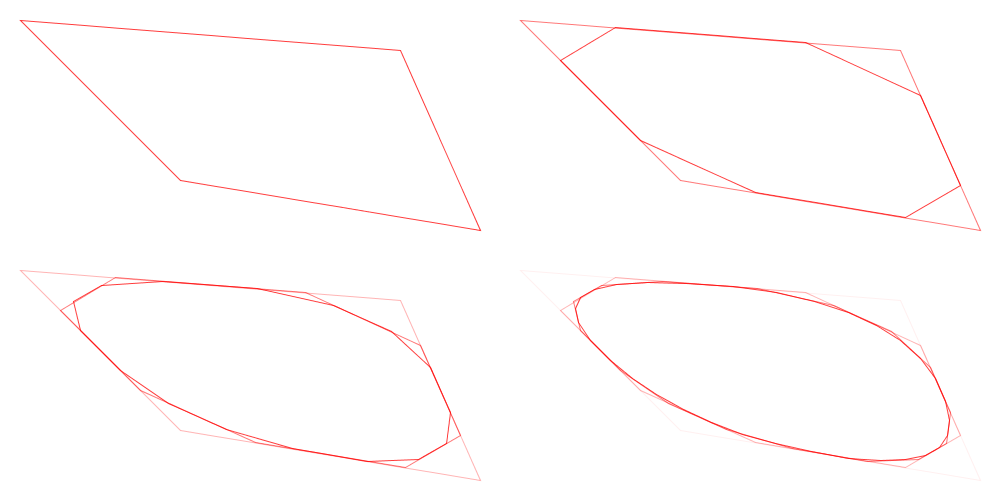
Animation of Chaikin’s Corner-Cutting Algorithm for a Closed Polygon

What Can I Do With Them?

Let’s now look at some ways you can incorporate Chaikin curves into your artwork.

Here is an example of using Chaikin’s corner-cutting algorithm to round out the polygons of a Voronoi diagram. As you can see, doing this gives a nice “cobbled” effect:

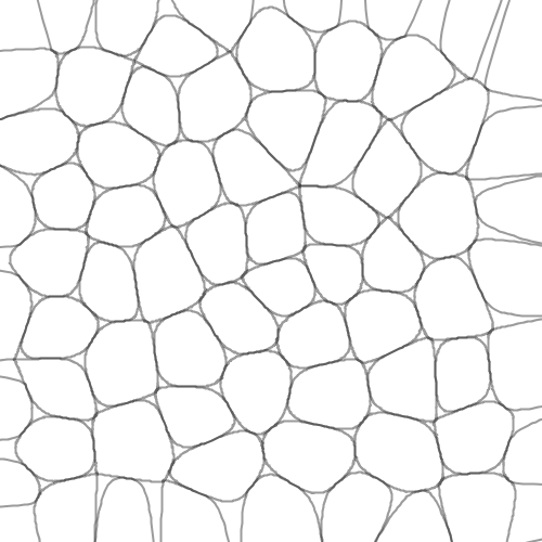
And here is the same image with the original Voronoi diagram overlaid on top in red, to show you how the rounding works:

Here is another example where you can use deformed polygons (i.e. a regular polygon with some random perturbation in each vertex) as an input to the Chaikin corner-cutting algorithm to produce blob-like shapes:

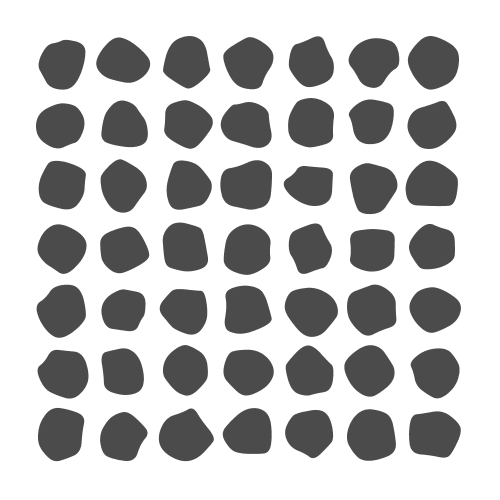
Here is a similar idea to generating blobs as above, but instead overlaying them on top of one another at a low opacity to give a soft edge:

Below is a texture created from a single Chaikin curve. A random walk is used to create a sequence of line segments as we jump around the canvas, and it’s smoothed out at the end using the corner-cutting algorithm:

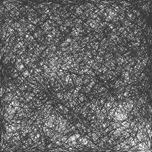
Here is a final example of creating a soft brush-like texture for your lines. Similar to the previous one, the image below uses a single set of points and applies a corner-cutting algorithm on it. However, I do this multiple times, with slight perturbations in the positions of the vertices each time.

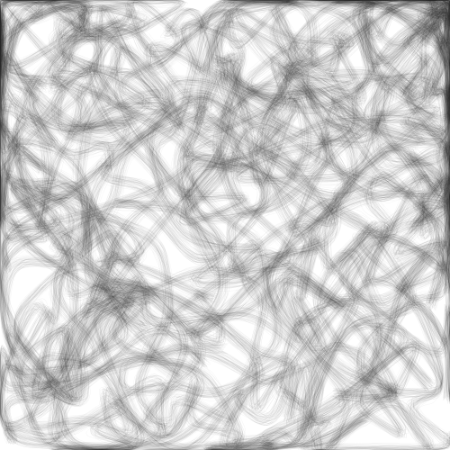
As you can see, the approach is fairly versatile and there are many ways you can incorporate Chaikin curves in your artwork! Let’s now look at how to implement this simple algorithm in Processing.

Implementation in Processing

Although the code I will show here is in Processing/Java, I want you to take away the following high-level algorithmic idea so you can implement it in any language of your choice.

High-Level Algorithm

The basic procedure for generating Chaikin curves is called the corner-cutting algorithm and looks something like this:

1. Given an initial shape (open or closed) in the form of a sequence of vertices
2. For each interior vertex forming a corner, replace it with two new vertices representing a cut.

Let’s try to implement this algorithm to better understand how it works.

Function Skeleton

Now let’s try to implement this in Processing! We first define an empty function as shown below:

/*
 * The following function takes as input a curve (in the form of
 * a PShape object), a cutting ratio, the number of iterations of
 * the corner-cutting algorithm to use, and a boolean specifying
 * whether the PShape provided is an open shape (e.g. line) or a
 * closed polygon (e.g. hexagon).
 */
PShape chaikin(PShape shape, float ratio, int iterations, boolean close) {
  PShape next = createShape();

  // Take the shape specified in the 'shape' variable and
  // generate a Chaikin version out of it inside 'next'.

  return next;
}

Above, we define an empty function the takes as input a PShape object. This is a handy way to store a shape comprising multiple vertices in Processing. We can use it to specify both open shapes (e.g. lines) as well as closed ones (i.e. polygons).

Since we’re going to be cutting the edges attached to each edge based on some fixed ratio, we take a ratio parameter that has a value between zero and one. For example, a ratio of 0.25 would mean cutting each edge one quarter and three quarters in.

Next, since we can run the cutting algorithm multiple times, we accept an iterations parameter specifying this number.

Finally, since our PShape might have been open or closed, and Processing provides no easy way to determine this, we take a boolean argument that lets us specify it manually.

Based on this, we can define two convenience functions to deal with open and closed shapes. The only difference in the functions below is the value of the last parameter passed to the chaikin() function call.

PShape chaikin_closed(PShape shape, float ratio, int iterations) {
  return chaikin(shape, ratio, iterations, true);
}

PShape chaikin_open(PShape shape, float ratio, int iterations) {
  return chaikin(shape, ratio, iterations, false);
}

A Recursive Algorithm

Now let’s get into the meat of it: how do we actually implement the corner-cutting algorithm?

Remember that Chaikin’s algorithm involves repeating the procedure a bunch of times (as specified by our iterations parameter). We can use recursion to achieve this; that is, we will call the chaikin() function from inside the chaikin() function itself:

PShape chaikin(PShape shape, float ratio, int iterations, boolean close) {
  // If the number of iterations is zero, return shape as is
    if (iterations == )
      return shape;

  PShape next = createShape();
  ...
  // Perform one iteration of the corner-cutting algorithm here.
  ...

  /*
   * Call the chaikin() function with one less iteration and our
   * newly-created shape so it's used as the new base shape. This
   * returns a PShape which we give back to the user.
   *
   */
  return chaikin(next, ratio, iterations - , close);
}

The above code is an example of a recursive call. Let’s ignore the first if statement for now and look below that. When we first invoke the chaikin() function in our code, we first create a new shape and apply one iteration of the corner-cutting algorithm.

Now we use this new shape as the basis for the next iteration! We return the result of a chaikin() function call, but pass it the new shape as a base and give tell it to perform one less iteration (since we already performed one).

This way, the shape gets refined over and over! However, we need to stop at some point and return the shape as it currently stands. This is done when we see that the chaikin() function was invoked with an iterations value of zero. This brings us to the first if statement: we check if the number of iterations hit zero and return the shape immediately (without performing another iteration).

Cutting a Corner

Let’s now leave our skeleton function as is for now and write a function to cut a single corner of our shape:

ArrayList<PVector> chaikin_cut(PVector a, PVector b, float ratio) {
  float x, y;
  ArrayList<PVector> n = new ArrayList<PVector>();

  /*
   * If ratio is greater than 0.5 flip it so we avoid cutting across
   * the midpoint of the line.
   */
   if (ratio > 0.5) ratio =  - ratio;

  /* Find point at a given ratio going from A to B */
  x = lerp(a.x, b.x, ratio);
  y = lerp(a.y, b.y, ratio);
  n.add(new PVector(x, y));

  /* Find point at a given ratio going from B to A */
  x = lerp(b.x, a.x, ratio);
  y = lerp(b.y, a.y, ratio);
  n.add(new PVector(x, y));

  return n;
}

Above, the function takes two vertices (as PVector’s) that represent a single edge of our shape, and a cut ratio between zero and one as seen before. From this, we derive two new points: one at the specified ratio when going from point A to point B, and one when going in the reverse direction. For example, cutting an edge with a ratio of 0.25 would give us two points: the first at 25% from point A and the other at 75% from point A (or 25% from point B).

You’ll notice an if condition that checks the value of ratio and inverts it if the value is greater than 0.5. This is required to avoid cutting across the midpoint of the edge, which would otherwise lead to an incorrect ordering of vertices in the final shape. This little if statement fixes that before we do all our calculations.

To calculate this, we use Processing’s lerp() function to interpolate the X and Y coordinates as shown above.

Finally, we add the two new points into an ArrayList and return it.

Drawing Into a PShape Object

Let’s now get back to the function we left off earlier and finish it up. Let’s first look at how we can draw inside a PShape in Processing:

PShape chaikin(PShape shape, float ratio, int iterations, boolean close) {
  ...
  PShape next = createShape();
  next.beginShape();

  // Draw the next iteration of the shape using corner cutting

  if (close)
    next.endShape(CLOSE);
  else
    next.endShape();

  return chaikin(next, ratio, iterations - , close);
}

In Processing, in order to draw inside a PShape object, we must first call its beginShape() function. Once all drawing operations have completed, we must call endShape(). For closed polygons, we must additionally pass the CLOSE parameter to endShape().

Above, we beginShape() after calling createShape(), and depending on whether we specified this to be an open or closed shape, call the appropriate endShape() version (i.e. with or without the CLOSE parameter).

Cutting Corners

Now let’s look at the main logic for creating the next iteration of a given shape using the corner-cutting algorithm:

PShape chaikin(PShape shape, float ratio, int iterations, boolean close) {
  ...
  next.beginShape();

  /*
   * Step 1: Figure out how many corners the shape has
   *         depending on whether it's open or closed.
   */
  int num_corners = shape.getVertexCount();
  if (!close)
    num_corners = shape.getVertexCount() - ;

  /*
   * Step 2: Since we don't have access to edges directly
   *         with a PShape object, do a pairwise iteration
   *         over vertices instead. Same thing.
   */
  for (int i = ; i < num_corners; i++) {

    // Get the i'th and (i+1)'th vertex to work on that edge.
    PVector a = shape.getVertex(i);
    PVector b = shape.getVertex((i + ) % shape.getVertexCount());

    // Step 3: Break it using our chaikin_cut() function
    ArrayList<PVector> n = chaikin_cut(a, b, ratio);

    /*
     * Now we have to deal with one corner case. In the case
     * of open shapes, the first and last endpoints shouldn't
     * be moved. However, in the case of closed shapes, we
     * cut all edges on both ends.
     */
    if (!close && i == ) {
      // For the first point of open shapes, ignore vertex A
      next.vertex(a.x, a.y);
      next.vertex(n.get().x, n.get().y);
    } else if (!close && i == num_corners - ) {
      // For the last point of open shapes, ignore vertex B
      next.vertex(n.get().x, n.get().y);
      next.vertex(b.x, b.y);
    } else {
      // For all other cases (i.e. interior edges of open
      // shapes or edges of closed shapes), add both vertices
      // returned by our chaikin_cut() method
      next.vertex(n.get().x, n.get().y);
      next.vertex(n.get().x, n.get().y);
    }
  }

  if (close)
    next.endShape(CLOSE);
  else
    next.endShape();

  return chaikin(next, ratio, iterations - , close);
}

The logic above can be broken into three steps. We first figure out how many corners the shape has depending on whether it’s open or closed. In closed shapes (e.g., rectangles or triangles) each vertex represents a corner, making the number of vertices is the same as the number of corners in it. In the case of open shapes, the number of edges is one less that the number of vertices (since the last vertex is not connected back to the first one).

The second step is to iterate over each edge. Unfortunately, Processing doesn’t provide any function to do this directly, so we iterate over vertices in a pairwise fashion instead. Above, we get the i^th and (i+1)^th vertex in each loop iteration. We also make sure, that for closed shapes, when we reach the end, we wrap around to pick the first vertex (using the modulo operator).

Finally, for each edge, we break it using out chaikin_cut() function. This returns two vertices by cutting off both ends of our edge. At this point we deal with one last corner case: we make sure that for open shapes, we don’t change the first and last vertices and keep the originals.

And that’s it!

Here’s our final implementation in a nice copy-pasteable snippet:

ArrayList<PVector> chaikin_cut(PVector a, PVector b, float ratio) {
  float x, y;
  ArrayList<PVector> n = new ArrayList<PVector>();

  /*
   * If ratio is greater than 0.5 flip it so we avoid cutting across
   * the midpoint of the line.
   */
   if (ratio > 0.5) ratio =  - ratio;

  /* Find point at a given ratio going from A to B */
  x = lerp(a.x, b.x, ratio);
  y = lerp(a.y, b.y, ratio);
  n.add(new PVector(x, y));

  /* Find point at a given ratio going from B to A */
  x = lerp(b.x, a.x, ratio);
  y = lerp(b.y, a.y, ratio);
  n.add(new PVector(x, y));

  return n;
}

PShape chaikin(PShape shape, float ratio, int iterations, boolean close) {
  // If the number of iterations is zero, return shape as is
  if (iterations == )
    return shape;

  PShape next = createShape();
  next.beginShape();

  /*
   * Step 1: Figure out how many corners the shape has
   *         depending on whether it's open or closed.
   */
  int num_corners = shape.getVertexCount();
  if (!close)
    num_corners = shape.getVertexCount() - ;

  /*
   * Step 2: Since we don't have access to edges directly
   *         with a PShape object, do a pairwise iteration
   *         over vertices instead. Same thing.
   */
  for (int i = ; i < num_corners; i++) {

    // Get the i'th and (i+1)'th vertex to work on that edge.
    PVector a = shape.getVertex(i);
    PVector b = shape.getVertex((i + ) % shape.getVertexCount());

    // Step 3: Break it using our chaikin_break() function
    ArrayList<PVector> n = chaikin_cut(a, b, ratio);

    /*
     * Now we have to deal with one corner case. In the case
     * of open shapes, the first and last endpoints shouldn't
     * be moved. However, in the case of closed shapes, we
     * cut all edges on both ends.
     */
    if (!close && i == ) {
      // For the first point of open shapes, ignore vertex A
      next.vertex(a.x, a.y);
      next.vertex(n.get().x, n.get().y);
    } else if (!close && i == num_corners - ) {
      // For the last point of open shapes, ignore vertex B
      next.vertex(n.get().x, n.get().y);
      next.vertex(b.x, b.y);
    } else {
      // For all other cases (i.e. interior edges of open
      // shapes or edges of closed shapes), add both vertices
      // returned by our chaikin_break() method
      next.vertex(n.get().x, n.get().y);
      next.vertex(n.get().x, n.get().y);
    }
  }

  if (close)
    next.endShape(CLOSE);
  else
    next.endShape();

  return chaikin(next, ratio, iterations - , close);
}

PShape chaikin_close(PShape original, float ratio, int iterations) {
  return chaikin(original, ratio, iterations, true);
}

PShape chaikin_open(PShape original, float ratio, int iterations) {
  return chaikin(original, ratio, iterations, false);
}