(转)Introduction to Gradient Descent Algorithm (along with variants) in Machine Learning
Introduction
Optimization is always the ultimate goal whether you are dealing with a real life problem or building a software product. I, as a computer science student, always fiddled with optimizing my code to the extent that I could brag about its fast execution.
Optimization basically means getting the optimal output for your problem. If you read the recent article on optimization, you would be acquainted with how optimization plays an important role in our real-life.
Optimization in machine learning has a slight difference. Generally, while optimizing, we know exactly how our data looks like and what areas we want to improve. But in machine learning we have no clue how our “new data” looks like, let alone try to optimize on it.
So in machine learning, we perform optimization on the training data and check its performance on a new validation data.
Broad applications of Optimization
There are various kinds of optimization techniques which are applied across various domains such as
- Mechanics – For eg: In deciding the surface of aerospace design
- Economics – For eg: Cost minimization
- Physics – For eg: Optimization time in quantum computing
Optimization has many more advanced applications like deciding optimal route for transportation, shelf-space optimization, etc.
Many popular machine algorithms depend upon optimization techniques such as linear regression, k-nearest neighbors, neural networks, etc. The applications of optimization are limitless and is a widely researched topic in both academia and industries.
In this article, we will look at a particular optimization technique called Gradient Descent. It is the most commonly used optimization technique when dealing with machine learning.
Table of Content
- What is Gradient Descent?
- Challenges in executing Gradient Descent
- Variants of Gradient Descent algorithm
- Implementation of Gradient Descent
- Practical tips on applying gradient descent
- Additional Resources
1. What is Gradient Descent?
To explain Gradient Descent I’ll use the classic mountaineering example.
Suppose you are at the top of a mountain, and you have to reach a lake which is at the lowest point of the mountain (a.k.a valley). A twist is that you are blindfolded and you have zero visibility to see where you are headed. So, what approach will you take to reach the lake?

The best way is to check the ground near you and observe where the land tends to descend. This will give an idea in what direction you should take your first step. If you follow the descending path, it is very likely you would reach the lake.
To represent this graphically, notice the below graph.

Let us now map this scenario in mathematical terms.
Suppose we want to find out the best parameters (θ1) and (θ2) for our learning algorithm. Similar to the analogy above, we see we find similar mountains and valleys when we plot our “cost space”. Cost space is nothing but how our algorithm would perform when we choose a particular value for a parameter.
So on the y-axis, we have the cost J(θ) against our parameters θ1 and θ2 on x-axis and z-axis respectively. Here, hills are represented by red region, which have high cost, and valleys are represented by blue region, which have low cost.
Now there are many types of gradient descent algorithms. They can be classified by two methods mainly:
- On the basis of data ingestion
- Full Batch Gradient Descent Algorithm
- Stochastic Gradient Descent Algorithm
In full batch gradient descent algorithms, you use whole data at once to compute the gradient, whereas in stochastic you take a sample while computing the gradient.
- On the basis of differentiation techniques
- First order Differentiation
- Second order Differentiation
Gradient descent requires calculation of gradient by differentiation of cost function. We can either use first order differentiation or second order differentiation.
2. Challenges in executing Gradient Descent
Gradient Descent is a sound technique which works in most of the cases. But there are many cases where gradient descent does not work properly or fails to work altogether. There are three main reasons when this would happen:
- Data challenges
- Gradient challenges
- Implementation challenges
2.1 Data Challenges
- If the data is arranged in a way that it poses a non-convex optimization problem. It is very difficult to perform optimization using gradient descent. Gradient descent only works for problems which have a well defined convex optimization problem.
- Even when optimizing a convex optimization problem, there may be numerous minimal points. The lowest point is called global minimum, whereas rest of the points are called local minima. Our aim is to go to global minimum while avoiding local minima.
- There is also a saddle point problem. This is a point in the data where the gradient is zero but is not an optimal point. We don’t have a specific way to avoid this point and is still an active area of research.
2.2 Gradient Challenges
- If the execution is not done properly while using gradient descent, it may lead to problems like vanishing gradient or exploding gradient problems. These problems occur when the gradient is too small or too large. And because of this problem the algorithms do not converge.
2.3 Implementation Challenges
- Most of the neural network practitioners don’t generally pay attention to implementation, but it’s very important to look at the resource utilization by networks. For eg: When implementing gradient descent, it is very important to note how many resources you would require. If the memory is too small for your application, then the network would fail.
- Also, its important to keep track of things like floating point considerations and hardware / software prerequisites.
3. Variants of Gradient Descent algorithms
Let us look at most commonly used gradient descent algorithms and their implementations.
3.1 Vanilla Gradient Descent
This is the simplest form of gradient descent technique. Here, vanilla means pure / without any adulteration. Its main feature is that we take small steps in the direction of the minima by taking gradient of the cost function.
Let’s look at its pseudocode.
update = learning_rate * gradient_of_parameters

parameters = parameters - update
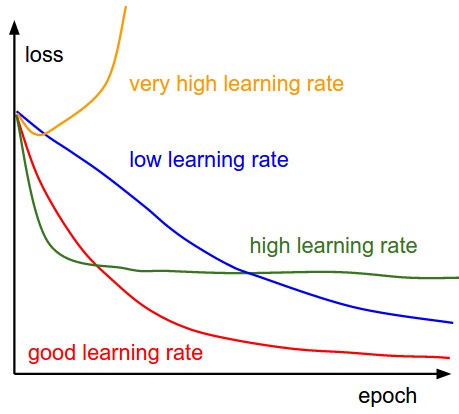
Here, we see that we make an update to the parameters by taking gradient of the parameters. And multiplying it by a learning rate, which is essentially a constant number suggesting how fast we want to go the minimum. Learning rate is a hyper-parameter and should be treated with care when choosing its value.
3.2 Gradient Descent with Momentum
Here, we tweak the above algorithm in such a way that we pay heed to the prior step before taking the next step.
Here’s a pseudocode.
update = learning_rate * gradient

velocity = previous_update * momentum

parameter = parameter + velocity – update
Here, our update is the same as that of vanilla gradient descent. But we introduce a new term called velocity, which considers the previous update and a constant which is called momentum.

3.3 ADAGRAD
ADAGRAD uses adaptive technique for learning rate updation. In this algorithm, on the basis of how the gradient has been changing for all the previous iterations we try to change the learning rate.
Here’s a pseudocode
grad_component = previous_grad_component + (gradient * gradient)

rate_change = square_root(grad_component) + epsilon

adapted_learning_rate = learning_rate * rate_change
update = adapted_learning_rate * gradient

parameter = parameter – update
In the above code, epsilon is a constant which is used to keep rate of change of learning rate in check.
3.4 ADAM
ADAM is one more adaptive technique which builds on adagrad and further reduces it downside. In other words, you can consider this as momentum + ADAGRAD.
Here’s a pseudocode.
adapted_gradient = previous_gradient + ((gradient – previous_gradient) * (1 – beta1))

gradient_component = (gradient_change – previous_learning_rate)

adapted_learning_rate =  previous_learning_rate + (gradient_component * (1 – beta2))
update = adapted_learning_rate * adapted_gradient

parameter = parameter – update
Here beta1 and beta2 are constants to keep changes in gradient and learning rate in check
There are also second order differentiation method like l-BFGS. You can see an implementation of this algorithm in scipy library.
4. Implementation of Gradient Descent
We will now look at a basic implementation of gradient descent using python.
Here we will use gradient descent optimization to find our best parameters for our deep learning model on an application of image recognition problem. Our problem is an image recognition, to identify digits from a given 28 x 28 image. We have a subset of images for training and the rest for testing our model. In this article we will take a look at how we define gradient descent and see how our algorithm performs. Referthis article for an end-to-end implementation using python.
Here is the main code for defining vanilla gradient descent,
params = [weights_hidden, weights_output, bias_hidden, bias_output]
def sgd(cost, params, lr=0.05):

  grads = T.grad(cost=cost, wrt=params)

  updates = []

  for p, g in zip(params, grads):

    updates.append([p, p - g * lr])

  return updates

updates = sgd(cost, params)
Now we break it down to understand it better.
We defined a function sgd with arguments as cost, params and lr. These represent J(θ) as seen previously, θ i.e. the parameters of our deep learning algorithm and our learning rate. We set default learning rate as 0.05, but this can be changed easily as per our preference.
def sgd(cost, params, lr=0.05):
We then defined gradients of our parameters with respect to the cost function. Here we used theano library to find gradients and we imported theano as T
grads = T.grad(cost=cost, wrt=params)
and finally iterated through all the parameters to find out the updates for all possible parameters. You can see that we use vanilla gradient descent here.
for p, g in zip(params, grads):

    updates.append([p, p - g * lr]
We can use this function to then find the best optimal parameters for our neural network. On using this function, we find that our neural network does a good enough job in finding the digits in our image as seen below
Prediction is: 8

In this implementation, we see that on using gradient descent we can get optimal parameters for our deep learning algorithm.
5. Practical tips on applying gradient descent
Each of the above mentioned gradient descent algorithms have their strengths and weaknesses. I’ll just mention some quick tips which might help you choose the right algorithm.
- For rapid prototyping, use adaptive techniques like Adam/Adagrad. These help in getting quicker results with much less efforts. As here, you don’t require much hyper-parameter tuning.
- To get the best results, you should use vanilla gradient descent or momentum. gradient descent is slow to get the desired results, but these results are mostly better than adaptive techniques.
- If your data is small and can be fit in a single iteration, you can use 2nd order techniques like l-BFGS. This is because 2nd order techniques are extremely fast and accurate, but are only feasible when data is small enough
- There also an emerging method (which I haven’t tried but looks promising) to use learned features to predict learning rates of gradient descent. Go through this paper for more details.
Now there are many reasons why a neural network fails to learn. But it helps immensely if you can monitor where your algorithm is going wrong.
When applying gradient descent, you can look at these points which might be helpful in circumventing the problem:
- Error rates – You should check the training and testing error after specific iterations and make sure both of them decreases. If that is not the case, there might be a problem!
- Gradient flow in hidden layers – Check if the network doesn’t show a vanishing gradient problem or exploding gradient problem.
- Learning rate – which you should check when using adaptive techniques.
6. Additional Resources
- Refer this paper on overview of gradient descent optimization algorithms.
- CS231n Course material on gradient descent.
- Chapter 4 (Numerical optimization) and Chapter 8 (Optimization for Deep Learning models) of Deep Learning book
End Notes
I hope you enjoyed reading this article. After going through this article, you will be adept with the basics of gradient descent and its variants. I have also given a practical tips for implementing them. Hope you found them helpful!
If you have any questions or doubts, feel free to post them in the comments below.
(转)Introduction to Gradient Descent Algorithm (along with variants) in Machine Learning的更多相关文章
- Introduction Of Gradient Descent
不是一个机器学习算法 是一种基于搜索的优化方法 作用:最小化一个损失函数 梯度上升法:最大化一个效用函数 import matplotlib.pyplot as plt import numpy as ...
- A Gentle Introduction to the Gradient Boosting Algorithm for Machine Learning
A Gentle Introduction to the Gradient Boosting Algorithm for Machine Learning by Jason Brownlee on S ...
- Logistic Regression and Gradient Descent
Logistic Regression and Gradient Descent Logistic regression is an excellent tool to know for classi ...
- flink 批量梯度下降算法线性回归参数求解(Linear Regression with BGD(batch gradient descent) )
1.线性回归 假设线性函数如下: 假设我们有10个样本x1,y1),(x2,y2).....(x10,y10),求解目标就是根据多个样本求解theta0和theta1的最优值. 什么样的θ最好的呢?最 ...
- (转) An overview of gradient descent optimization algorithms
An overview of gradient descent optimization algorithms Table of contents: Gradient descent variants ...
- An overview of gradient descent optimization algorithms
原文地址:An overview of gradient descent optimization algorithms An overview of gradient descent optimiz ...
- 【论文翻译】An overiview of gradient descent optimization algorithms
这篇论文最早是一篇2016年1月16日发表在Sebastian Ruder的博客.本文主要工作是对这篇论文与李宏毅课程相关的核心部分进行翻译. 论文全文翻译: An overview of gradi ...
- FITTING A MODEL VIA CLOSED-FORM EQUATIONS VS. GRADIENT DESCENT VS STOCHASTIC GRADIENT DESCENT VS MINI-BATCH LEARNING. WHAT IS THE DIFFERENCE?
FITTING A MODEL VIA CLOSED-FORM EQUATIONS VS. GRADIENT DESCENT VS STOCHASTIC GRADIENT DESCENT VS MIN ...
- 采用梯度下降优化器(Gradient Descent optimizer)结合禁忌搜索(Tabu Search)求解矩阵的全部特征值和特征向量
[前言] 对于矩阵(Matrix)的特征值(Eigens)求解,采用数值分析(Number Analysis)的方法有一些,我熟知的是针对实对称矩阵(Real Symmetric Matrix)的特征 ...
随机推荐
- 20155228 2016-2017-2 《Java程序设计》第1周学习总结
20155228 2016-2017-2 <Java程序设计>第1周学习总结 教材学习内容总结 这部分内容是以教材为基础,根据个人的理解来描述的,有的地方的理解和表述可能不规范甚至不正确, ...
- Spark学习之路 (三)Spark之RDD
一.RDD的概述 1.1 什么是RDD? RDD(Resilient Distributed Dataset)叫做弹性分布式数据集,是Spark中最基本的数据抽象,它代表一个不可变.可分区.里面的元素 ...
- 大数据处理框架之Strom:认识storm
Storm是分布式实时计算系统,用于数据的实时分析.持续计算,分布式RPC等. (备注:5种常见的大数据处理框架:· 仅批处理框架:Apache Hadoop:· 仅流处理框架:Apache Stor ...
- kali长时间未使用导致数字签名过期无法更新源解决办法
kali长时间未使用,数字签名会过期,从而导致无法更新源. apt-get update:从源(Source)服务器那里下载最新的软件包列: apt-get upgrade:对已经安装的软件包本身进行 ...
- 第三方包源码maven 下载
1,maven导包时候自动下载源码 在eclipse或者Myeclipse中 => window ==> preference ==> Maven ==> 勾选Download ...
- git使用遇到的坑
把一个完整项目提交到github上步骤以及注意事项 Git的安装就不说了. 第一步:mkdir/cd 我们需要先创建一个本地的版本库(其实也就是一个文件夹). 你可以直接右击新建文件夹,也可以右击打开 ...
- vue之vue-cookies安装和使用说明
vue之vue-cookies安装和使用说明npm官方链接:https://www.npmjs.com/package/vue-cookies 安装,在对应项目根目录下执行:npm install v ...
- tomcat1章1
package ex01.pyrmont; import java.net.Socket; import java.net.ServerSocket; import java.net.InetAddr ...
- 关于Ajax无法下载文件到浏览器本地的问题
最近在做网站的时候遇到这样一个功能,在如图所示的页面中,需要用户点击链接的时候,能够以异步Ajax的方式判断服务器中是否存储有相应的Excel文件,如果没有的话就提示用户没有找到,如果有的话就下载到用 ...
- css技巧-案例
点击进入:http://herry.wuhairui.cn/cssSkill/main.html