二分类模型之logistic

liner classifiers

逻辑回归用在2分类问题上居多。它是一个非线性的回归模型，其最大的好处恰恰是可以解决二元类问题，目前在金融行业，基本都是使用Logistic回归来预判一个用户是否为好客户，因为它还弥补了其他黑盒模型（SVM、神经网络、随机森林等）不具解释性的缺点。知乎

1.logistic

• 逻辑回归其实是一个分类算法而不是回归算法。通常是利用已知的自变量来预测一个离散型因变量的值（像二进制值0/1，是/否，真/假）。简单来说，它就是通过拟合一个逻辑函数（logit fuction）来预测一个事件发生的概率。所以它预测的是一个概率值，自然，它的输出值应该在0到1之间。--计算的是单个输出

1.2 sigmoid

逻辑函数

\(g(z)=\frac{1}{1+e^{-z}}\)

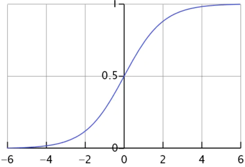
• sigmoid函数是一个s形的曲线，它的取值在[0, 1]之间，在远离0的地方函数的值会很快接近0或者1。它的这个特性对于解决二分类问题十分重要
• 二分类中，输出y的取值只能为0或者1，所以在线性回归的假设函数外包裹一层Sigmoid函数，使之取值范围属于(0,1)，完成了从值到概率的转换。逻辑回归的假设函数形式如下
  
  \(h_{\theta}(x)=g\left(\theta^{T} x\right)=\frac{1}{1+e^{-\theta^{T} x}}=P(y=1 | x ; \theta)\)
  
  则若\(P(y=1 | x ; \theta)=0.7\)，则表示输入为x的时候，y=1的概率为0.7

1.3 决策边界

决策边界，也称为决策面，是用于在N维空间，将不同类别样本分开的直线或曲线，平面或曲面

根据以上假设函数表示概率，我们可以推得

if \(h_{\theta}(x) \geqslant 0.5 \Rightarrow y=1\)

if \(h_{\theta}(x)<0.5 \Rightarrow y=0\)

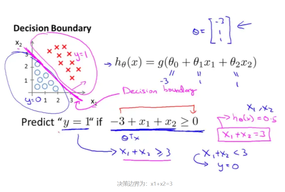
1.3.1 线性决策边界

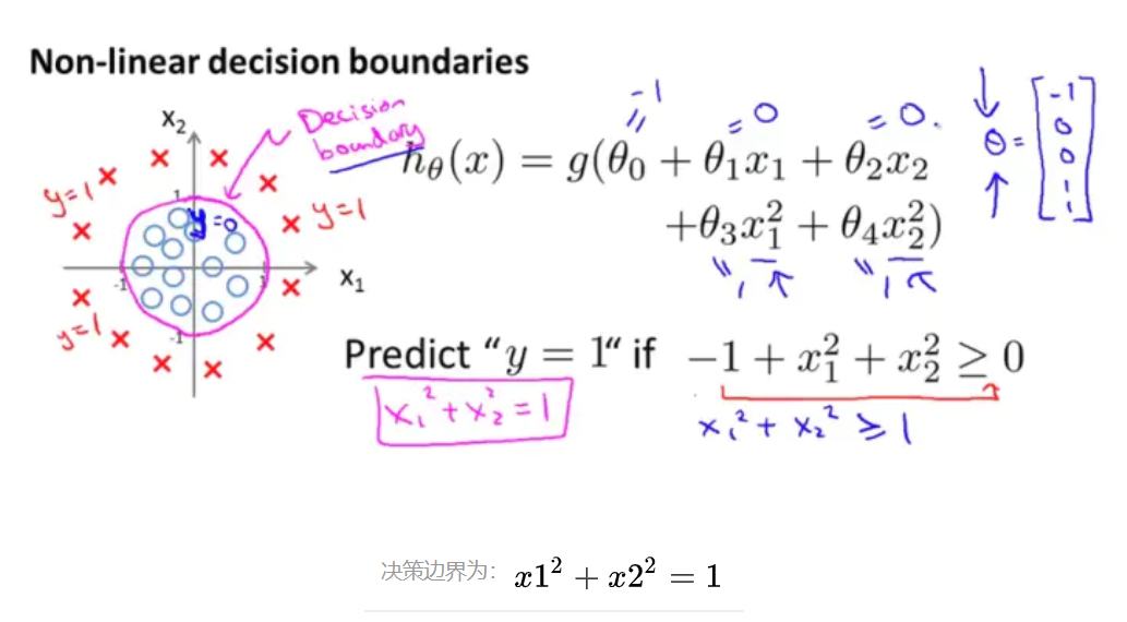
1.3.2 非线性决策边界

1.4 代价函数/损失函数

在线性回归中的代价函数为

\(J(\theta)=\frac{1}{2 m} \sum_{i=1}^{m}\left(h_{\theta}\left(x^{(i)}\right)-y^{(i)}\right)^{2}\)

• 因为它是一个凸函数，所以可用梯度下降直接求解，局部最小值即全局最小值
• 只有把函数是或者转化为凸函数，才能使用梯度下降法进行求导哦
• 在逻辑回归中，\(h_{\theta }(x)\)是一个复杂的非线性函数，属于非凸函数，直接使用梯度下降会陷入局部最小值中。类似于线性回归，逻辑回归的\(J(\theta )\)的具体求解过程如下
• 对于输入x，分类结果为类别1和类别0的概率分别为:
  
  \(P(y=1 | x ; \theta)=h(x) ; \quad P(y=0 | x ; \theta)=1-h(x)\)
• 因此化简为一个式子可以写为
  
  \(\left.P(y | x ; \theta)=(h(x))^{y}(1-h(x))^{(} 1-y\right)\)

1.4.1 似然函数

\(\begin{aligned} L(\theta) &=\prod_{i=1}^{m} P\left(y^{(i)} | x^{(i)} ; \theta\right) \\ &=\prod_{i=1}^{m}\left(h_{\theta}\left(x^{(i)}\right)\right)^{y^{(0)}}\left(1-h_{\theta}\left(x^{(i)}\right)\right)^{1-y^{(i)}} \end{aligned}\)

似然函数取对数之后

\(\begin{aligned} l(\theta) &=\log L(\theta) \\ &=\sum_{i=1}^{m}\left(y^{(i)} \log h_{\theta}\left(x^{(i)}\right)+\left(1-y^{(i)}\right) \log \left(1-h_{\theta}\left(x^{(i)}\right)\right)\right) \end{aligned}\)

• 根据最大似然估计，需要使用梯度上升法求最大值，因此，为例能够使用梯度下降法，需要将代价函数构造成为凸函数
  
  因此
  
  \(J(\theta )=-\frac{1}{m} l(\theta )\)
  
  此时可以使用梯度下降求解了
• \(\theta_{j}\)更新过程为
  
  \(\theta_{j}:=\theta_{j}-\alpha \frac{\partial}{\partial \theta_{j}} J(\theta)\)
  
  中间求导过程省略
  
  \(\theta_{j}:=\theta_{j}-\alpha \frac{1}{m} \sum_{i=1}^{m}\left(h_{\theta}\left(\mathrm{x}^{(i)}\right)-y^{(i)}\right) x_{j}^{(i)}, \quad(j=0 \ldots n)\)

1.5正则化

损失函数中增加惩罚项：参数值越大惩罚越大–>让算法去尽量减少参数值

损失函数 \(J(β)\)的简写形式:

\(J(\beta)=\frac{1}{m} \sum_{i=1}^{m} \cos (y, \beta)+\frac{\lambda}{2 m} \sum_{j=1}^{n} \beta_{j}^{2}\)

• 当模型参数 β 过多时，损失函数会很大，算法要努力减少 β 参数值来让损失函数最小。
• λ 正则项重要参数，λ 越大惩罚越厉害，模型越欠拟合，反之则倾向过拟合

1.5.1 lasso

l1正则化

\(J(\beta)=\frac{1}{m} \sum_{i=1}^{\mathrm{m}} \cos t(y, \beta)+\frac{\lambda}{2 m} \sum_{j=1}^{n}\left|\beta_{j}\right|\)

1.5.2 ridge

l2正则化

\(J(\beta)=\frac{1}{m} \sum_{i=1}^{\mathrm{m}} \cos t(y, \beta)+\frac{\lambda}{2 m} \sum_{j=1}^{n} \beta_{j}^{2}\)

1.6 python实现

class sklearn.linear_model.LogisticRegression(penalty='l2', dual=False, tol=0.0001, C=1.0, fit_intercept=True, intercept_scaling=1, class_weight=None, random_state=None, solver='lbfgs', max_iter=100, multi_class='auto', verbose=0, warm_start=False, n_jobs=None, l1_ratio=None

1.6.1 参数

• penalty：{‘l1’, ‘l2’, ‘elasticnet’, ‘none’}, default=’l2’ 正则项，默认是l2
  • The ‘newton-cg’, ‘sag’ and ‘lbfgs’ solvers support only l2 penalties. ‘elasticnet’ is only supported by the ‘saga’ solver. If ‘none’ (not supported by the liblinear solver), no regularization is applied.LogisticRegression
• dual：bool, default=False
  
  -Dual formulation is only implemented for l2 penalty with liblinear solver. Prefer dual=False when n_samples > n_features，一般情况下是false
• tol：float, default=1e-4 阈值，迭代终止条件按
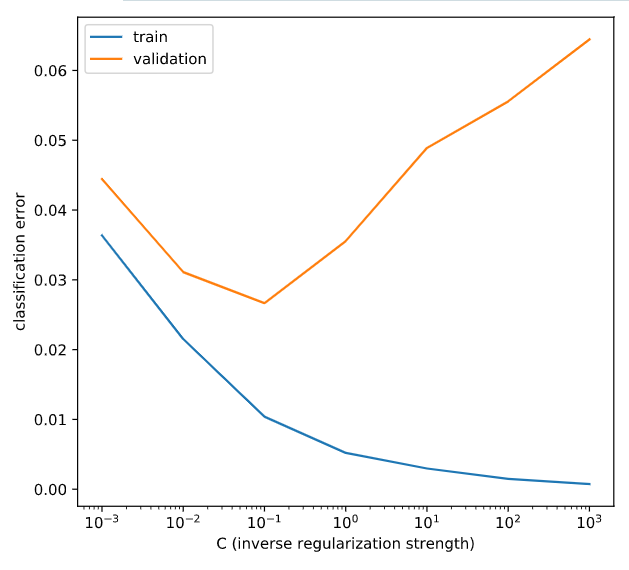
• C：float, default=1.0
  • Inverse of regularization strength; must be a positive float. Like in support vector machines, smaller values specify stronger regularization，正则化强度的倒数；必须是正浮点数。与支持向量机一样，较小的值指定更强的正则化
    
    -solver：{‘newton-cg’, ‘lbfgs’, ‘liblinear’, ‘sag’, ‘saga’}, default=’lbfgs’
  • Algorithm to use in the optimization problem.
  • For small datasets, ‘liblinear’ is a good choice, whereas ‘sag’ and ‘saga’ are faster for large ones.
  • For multiclass problems, only ‘newton-cg’, ‘sag’, ‘saga’ and ‘lbfgs’ handle multinomial loss; ‘liblinear’ is limited to one-versus-rest schemes.
  • ‘newton-cg’, ‘lbfgs’, ‘sag’ and ‘saga’ handle L2 or no penalty
  • ‘liblinear’ and ‘saga’ also handle L1 penalty
  • ‘saga’ also supports ‘elasticnet’ penalty
  • ‘liblinear’ does not support setting penalty='none'
• multi_class：{‘auto’, ‘ovr’, ‘multinomial’}, default=’auto’ 这个参数是多元分类中用到的，二分类中不涉及
  • If the option chosen is ‘ovr’, then a binary problem is fit for each label.
  • For ‘multinomial’ the loss minimised is the multinomial loss fit across the entire probability distribution, even when the data is binary. **‘multinomial’ is unavailable when solver=’liblinear’. **
    
    -‘auto’ selects ‘ovr’ if the data is binary, or if solver=’liblinear’, and otherwise selects ‘multinomial’.

1.6.1 属性

• classes_：ndarray of shape (n_classes, )属性数组
  
  A list of class labels known to the classifier.
• coef_：ndarray of shape (1, n_features) or (n_classes, n_features)属性和特征分类的数组
  • Coefficient of the features in the decision function.
  • coef_ is of shape (1, n_features) when the given problem is binary. In particular, when multi_class='multinomial', coef_ corresponds to outcome 1 (True) and -coef_ corresponds to outcome 0 (False).
• intercept_：ndarray of shape (1,) or (n_classes,)
  
  Intercept (a.k.a. bias) added to the decision function.
  
  If fit_intercept is set to False, the intercept is set to zero. intercept_ is of shape (1,) when the given problem is binary. In particular, when multi_class='multinomial', intercept_ corresponds to outcome 1 (True) and -intercept_ corresponds to outcome 0 (False).

n_iter_：ndarray of shape (n_classes,) or (1, )

Actual number of iterations for all classes. If binary or multinomial, it returns only 1 element. For liblinear solver, only the maximum number of iteration across all classes is given.

 # Create LogisticRegression object and fit
    lr = LogisticRegression(C=C_value)
    lr.fit(X_train, y_train)

    # Evaluate error rates and append to lists
    train_errs.append( 1.0 - lr.score(X_train, y_train) )
    valid_errs.append( 1.0 - lr.score(X_valid, y_valid) )

# Plot results
plt.semilogx(C_values, train_errs, C_values, valid_errs)
plt.legend(("train", "validation"))
plt.show()