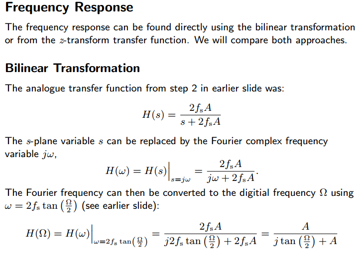
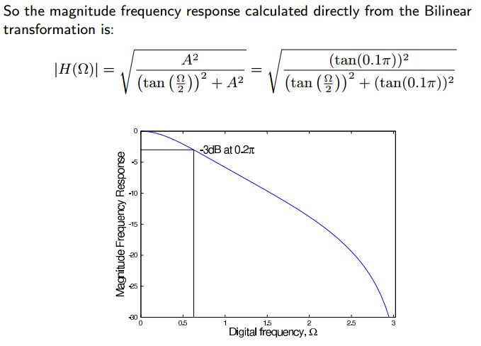
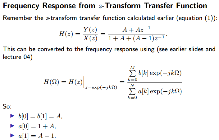
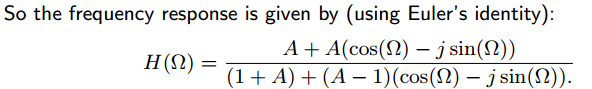
IIR filter design from analog filter

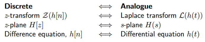
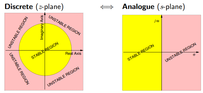
Analog filter和digital filter的联系：

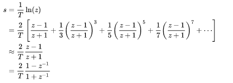
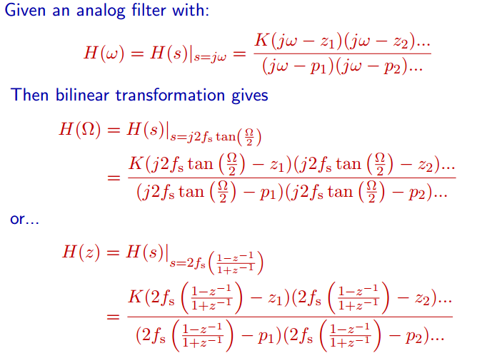
z变换与Laplace从数学上的关系为：

但这种关系在实际应用上不好实现，因此通常使用biliner transform(https://en.wikipedia.org/wiki/Bilinear_transform)来简化这种关系。

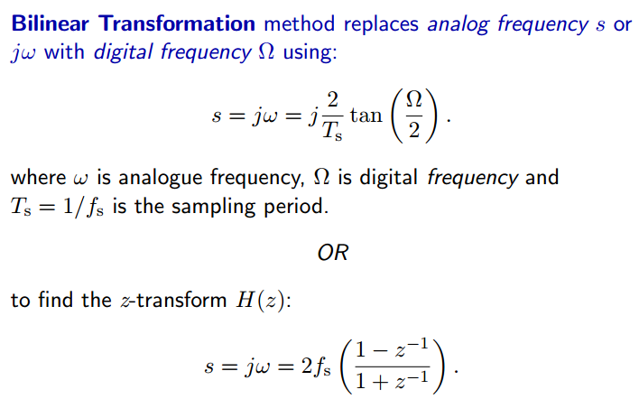
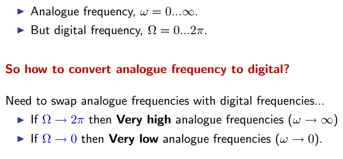
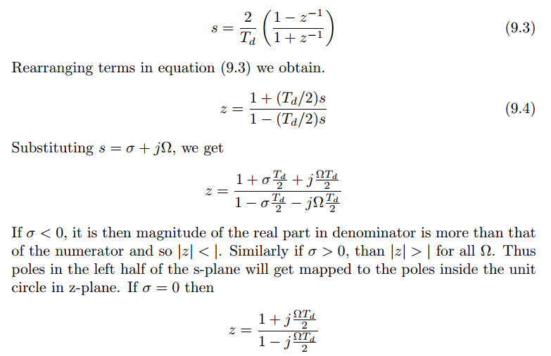
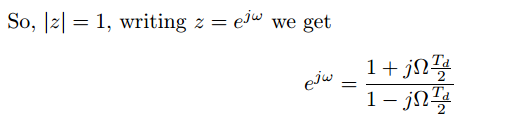
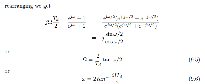
analog frequecy 和digital frequecy的联系推导过程如下：

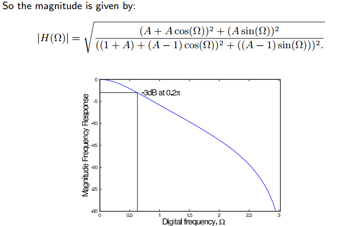
因此给定一个analog filter的传递函数，通过bilinear transform我们可以得到响应digital filter的频率响应和z变换

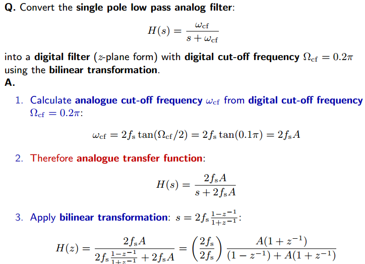
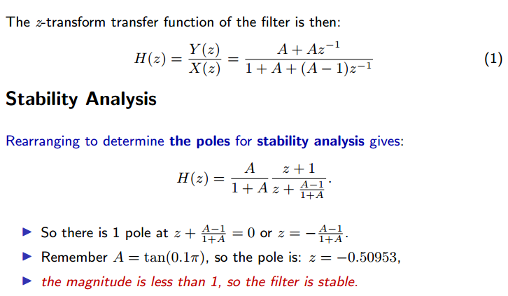
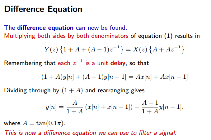
下面是一个例子：

https://ww2.mathworks.cn/help/signal/ug/iir-filter-design.html

Classical IIR Filter Design Using Analog Prototyping

The principal IIR digital filter design technique this toolbox provides is based on the conversion of classical lowpass analog filters to their digital equivalents. The following sections describe how to design filters and summarize the characteristics of the supported filter types. See Special Topics in IIR Filter Designfor detailed steps on  the filter design process.

Complete Classical IIR Filter Design

You can easily create a filter of any order with a lowpass, highpass, bandpass, or bandstop configuration using the filter design functions.

Filter Design Functions

Filter Type	Design Function
Bessel (analog only)	[b,a] = besself(n,Wn,options) [z,p,k] = besself(n,Wn,options) [A,B,C,D] = besself(n,Wn,options)
Butterworth	[b,a] = butter(n,Wn,options) [z,p,k] = butter(n,Wn,options) [A,B,C,D] = butter(n,Wn,options)
Chebyshev Type I	[b,a] = cheby1(n,Rp,Wn,options) [z,p,k] = cheby1(n,Rp,Wn,options) [A,B,C,D] = cheby1(n,Rp,Wn,options)
Chebyshev Type II	[b,a] = cheby2(n,Rs,Wn,options) [z,p,k] = cheby2(n,Rs,Wn,options) [A,B,C,D] = cheby2(n,Rs,Wn,options)
Elliptic	[b,a] = ellip(n,Rp,Rs,Wn,options) [z,p,k] = ellip(n,Rp,Rs,Wn,options) [A,B,C,D] = ellip(n,Rp,Rs,Wn,options)

By default, each of these functions returns a lowpass filter; you need to specify only the cutoff frequency that you want, Wn, in normalized units such that the Nyquist frequency is 1 Hz). For a highpass filter, append 'high' to the function's parameter list. For a bandpass or bandstop filter, specify Wn as a two-element vector containing the passband edge frequencies. Append 'stop' for the bandstop configuration.

Here are some example digital filters:

[b,a] = butter(5,0.4);                    % Lowpass Butterworth
[b,a] = cheby1(4,1,[0.4 0.7]);            % Bandpass Chebyshev Type I
[b,a] = cheby2(6,60,0.8,'high');          % Highpass Chebyshev Type II
[b,a] = ellip(3,1,60,[0.4 0.7],'stop');   % Bandstop elliptic

To design an analog filter, perhaps for simulation, use a trailing 's' and specify cutoff frequencies in rad/s:

[b,a] = butter(5,0.4,'s');      % Analog Butterworth filter

All filter design functions return a filter in the transfer function, zero-pole-gain, or state-space linear system model representation, depending on how many output arguments are present. In general, you should avoid using the transfer function form because numerical problems caused by roundoff errors can occur. Instead, use the zero-pole-gain form which you can convert to a second-order section (SOS) form using zp2sos and then use the SOS form to analyze or implement your filter.

Note

All classical IIR lowpass filters are ill-conditioned for extremely low cutoff frequencies. Therefore, instead of designing a lowpass IIR filter with a very narrow passband, it can be better to design a wider passband and decimate the input signal.

Designing IIR Filters to Frequency Domain Specifications

This toolbox provides order selection functions that calculate the minimum filter order that meets a given set of requirements.

Filter Type	Order Estimation Function
Butterworth	[n,Wn] = buttord(Wp,Ws,Rp,Rs)
Chebyshev Type I	[n,Wn] = cheb1ord(Wp,Ws,Rp,Rs)
Chebyshev Type II	[n,Wn] = cheb2ord(Wp,Ws,Rp,Rs)
Elliptic	[n,Wn] = ellipord(Wp,Ws,Rp,Rs)

These are useful in conjunction with the filter design functions. Suppose you want a bandpass filter with a passband from 1000 to 2000 Hz, stopbands starting 500 Hz away on either side, a 10 kHz sampling frequency, at most 1 dB of passband ripple, and at least 60 dB of stopband attenuation. You can meet these specifications by using the butter function as follows.

[n,Wn] = buttord([1000 2000]/5000,[500 2500]/5000,1,60)
[b,a] = butter(n,Wn);

n =
    12
Wn =
    0.1951    0.4080

An elliptic filter that meets the same requirements is given by

[n,Wn] = ellipord([1000 2000]/5000,[500 2500]/5000,1,60)
[b,a] = ellip(n,1,60,Wn);

n =
    5
Wn =
    0.2000    0.4000

These functions also work with the other standard band configurations, as well as for analog filters.

Comparison of Classical IIR Filter Types

The toolbox provides five different types of classical IIR filters, each optimal in some way. This section shows the basic analog prototype form for each and summarizes major characteristics.

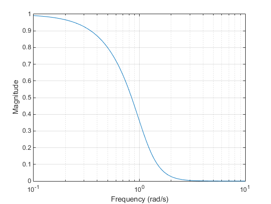
Butterworth Filter

The Butterworth filter provides the best Taylor series approximation to the ideal lowpass filter response at analog frequencies Ω  = 0 and Ω = ∞; for any order N, the magnitude squared response has 2N – 1 zero derivatives at these locations (maximally flat at Ω = 0 and Ω = ∞). Response is monotonic overall, decreasing smoothly from Ω = 0 to Ω = ∞. H(jΩ)=1/G2 at Ω = 1.

Chebyshev Type I Filter

The Chebyshev Type I filter minimizes the absolute difference between the ideal and actual frequency response over the entire passband by incorporating an equal ripple of Rp dB in the passband. Stopband response is maximally flat. The transition from passband to stopband is more rapid than for the Butterworth filter. H(jΩ)=10−Rp/20 at Ω = 1.

Chebyshev Type II Filter

The Chebyshev Type II filter minimizes the absolute difference between the ideal and actual frequency response over the entire stopband by incorporating an equal ripple of Rs dB in the stopband. Passband response is maximally flat.

The stopband does not approach zero as quickly as the type I filter (and does not approach zero at all for even-valued filter order n). The absence of ripple in the passband, however, is often an important advantage. H(jΩ)=10−Rs/20 at Ω = 1.

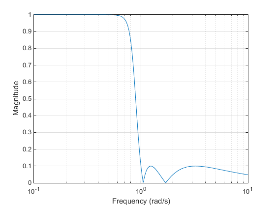
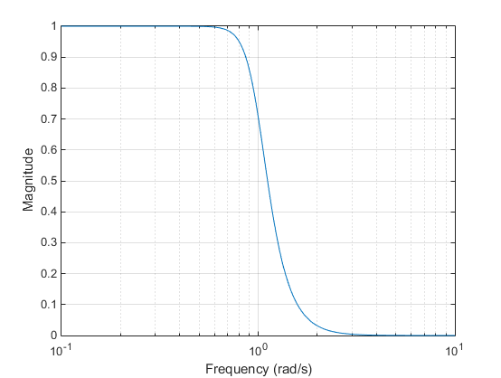
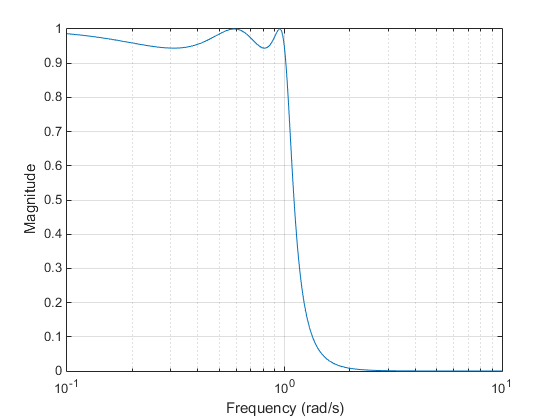
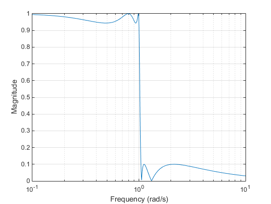
Elliptic Filter

Elliptic filters are equiripple in both the passband and stopband. They generally meet filter requirements with the lowest order of any supported filter type. Given a filter order n, passband ripple Rp in decibels, and stopband ripple Rs in decibels, elliptic filters minimize transition width. H(jΩ)=10−Rp/20 at Ω = 1.

Bessel Filter

Analog Bessel lowpass filters have maximally flat group delay at zero frequency and retain nearly constant group delay across the entire passband. Filtered signals therefore maintain their waveshapes in the passband frequency range. Frequency mapped and digital Bessel filters, however, do not have this maximally flat property; this toolbox supports only the analog case for the complete Bessel filter design function.

Bessel filters generally require a higher filter order than other filters for satisfactory stopband attenuation. H(jΩ)<1/G2 at Ω = 1 and decreases as filter order n increases.

Note

The lowpass filters shown above were created with the analog prototype functions besselap, buttap, cheb1ap, cheb2ap, and ellipap. These functions find the zeros, poles, and gain of an nth-order analog filter of the appropriate type with a cutoff frequency of 1 rad/s. The complete filter design functions (besself, butter, cheby1, cheby2, and ellip) call the prototyping functions as a first step in the design process. See Special Topics in IIR Filter Design for details.

To create similar plots, use n = 5 and, as needed, Rp = 0.5 and Rs = 20. For example, to create the elliptic filter plot:

[z,p,k] = ellipap(5,0.5,20);
w = logspace(-1,1,1000);
h = freqs(k*poly(z),poly(p),w);
semilogx(w,abs(h)), grid
xlabel('Frequency (rad/s)')
ylabel('Magnitude')

Direct IIR Filter Design

This toolbox uses the term direct methods to describe techniques for IIR design that find a filter based on specifications in the discrete domain. Unlike the analog prototyping method, direct design methods are not constrained to the standard lowpass, highpass, bandpass, or bandstop configurations. Rather, these functions design filters with an arbitrary, perhaps multiband, frequency response. This section discusses the yulewalk function, which is intended specifically for filter design; Parametric Modeling discusses other methods that may also be considered direct, such as Prony's method, Linear Prediction, the Steiglitz-McBride method, and inverse frequency design.

The yulewalk function designs recursive IIR digital filters by fitting a specified frequency response. yulewalk's name reflects its method for finding the filter's denominator coefficients: it finds the inverse FFT of the ideal specified magnitude-squared response and solves the modified Yule-Walker equations using the resulting autocorrelation function samples. The statement

[b,a] = yulewalk(n,f,m)

returns row vectors b and a containing the n+1 numerator and denominator coefficients of the nth-order IIR filter whose frequency-magnitude characteristics approximate those given in vectors f and m. f is a vector of frequency points ranging from 0 to 1, where 1 represents the Nyquist frequency. mis a vector containing the specified magnitude response at the points in f. f and m can describe any piecewise linear shape magnitude response, including a multiband response. The FIR counterpart of this function is fir2, which also designs a filter based on an arbitrary piecewise linear magnitude response. See FIR Filter Design for details.

Note that yulewalk does not accept phase information, and no statements are made about the optimality of the resulting filter.

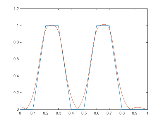
Design a multiband filter with yulewalk and plot the specified and actual frequency response:

m = [0   0   1   1   0   0   1   1   0 0];
f = [0 0.1 0.2 0.3 0.4 0.5 0.6 0.7 0.8 1];
[b,a] = yulewalk(10,f,m);
[h,w] = freqz(b,a,128)
plot(f,m,w/pi,abs(h))

Generalized Butterworth Filter Design

The toolbox function maxflat enables you to design generalized Butterworth filters, that is, Butterworth filters with differing numbers of zeros and poles. This is desirable in some implementations where poles are more expensive computationally than zeros. maxflat is just like the butter function, except that it you can specify two orders (one for the numerator and one for the denominator) instead of just one. These filters are maximally flat. This means that the resulting filter is optimal for any numerator and denominator orders, with the maximum number of derivatives at 0 and the Nyquist frequency ω = π both set to 0.

For example, when the two orders are the same, maxflat is the same as butter:

[b,a] = maxflat(3,3,0.25)

b =
    0.0317    0.0951    0.0951    0.0317
a =
    1.0000   -1.4590    0.9104   -0.1978

[b,a] = butter(3,0.25)

b =
    0.0317    0.0951    0.0951    0.0317
a =
    1.0000   -1.4590    0.9104   -0.1978

However, maxflat is more versatile because it allows you to design a filter with more zeros than poles:

[b,a] = maxflat(3,1,0.25)

b =
    0.0950    0.2849    0.2849    0.0950
a =
    1.0000   -0.2402

The third input to maxflat is the half-power frequency, a frequency between 0 and 1 with a magnitude response of 1/G2.

You can also design linear phase filters that have the maximally flat property using the 'sym' option:

maxflat(4,'sym',0.3)

ans =
    0.0331    0.2500    0.4337    0.2500    0.0331

For complete details of the maxflat algorithm, see Selesnick and Burrus [2].