A Statistical View of Deep Learning (V): Generalisation and Regularisation

We now routinely build complex, highly-parameterised models in an effort to address the complexities of modern data sets. We design our models so that they have enough 'capacity', and this is now second nature to us using the layer-wise design principles of deep learning. But some problems continue to affect us, those that we encountered even in the low-data regime, the problem of overfitting and seeking better generalisation.

The classical description of deep feedforward networks in part I or of recurrent networks inpart IV established maximum likelihood as the the underlying estimation principle for these models. Maximum Likelihood (ML) [1] is an elegant, conceptually simple and easy to implement estimation framework. And it has several statistical advantages, including consistency and asymptotic efficiency. Deep learning has shown just how effective ML can be. But it is not without its disadvantages, the most prominent being a tendency for overfitting. Overfitting is the problem of all statistical sciences, and ways of dealing with this are abound. The general solution reduces to considering an estimation framework other than maximum likelihood — this penultimate post explores some of the available alternatives.

Regularisers and Priors

The principle technique for addressing overfitting in deep learning is by regularisation — adding additional penalties to our training objective that prevents the model parameters from becoming large and from fitting to the idiosyncrasies of the training data. This transforms our estimation framework from maximum likelihood into amaximum penalised likelihood, or more commonly maximum a posteriori (MAP) estimation (or a shrinkage estimator). For a deep model with loss function L(θ) and parameters θ, we instead use the modified loss that includes a regularisation function R:

L(θ)=−∑nlogp(yn|xn,θ)+1λR(θ)

λ is a regularisation coefficient that is a hyperparameter of the model. It is also commonly known that this formulation can be derived by considering a probabilistic model that instead of a penalty, introduces a prior probability distribution over the parameters. The loss function is the negative of the log joint probability distribution:

logp(y,θ)=∑nlogp(yn|xn,θ)+logp(θ|λ)

The table shows some common regularisers, of which the L1 and L2 penalties are used in deep learning. Most other regularisers in the probabilistic literature cannot be added as a simple penalty function, but are instead given by a hierarchical specification (and whose optimisation is also more involved, requiring some form of alternating optimisation). Amongst the most effective are the sparsity inducing penalties such as Automatic Relevance Determination, the Normal-Inverse Gaussian, the Horseshoe, and the general class of Gaussian scale-mixtures.

Name	R(θ)	p(θ)
L2/Gaussian/Weight Decay	1λ∥θ∥22	N(θ\|0;λ)
L1/Laplace/Lasso	1λ∥θ∥1	Lap(θ\|0;λ)
p-norms	∥θ∥p;p>0	exp(−λ∥θ∥p)
Total variation	λ\|Δθ\|;Δθ=(θj−θj−1)
Fused Lasso	α\|θ\|+β\|Δθ\|
Cauchy	−∑ilog(θ2i+γ2)	1πγγ2(θ−μ)2+γ2

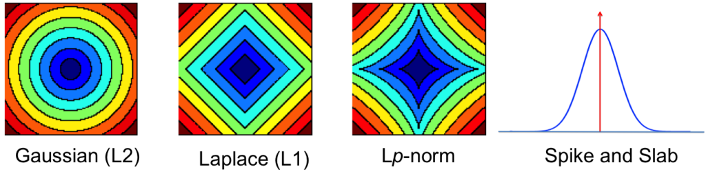
Contours showing the shrinkage effects of different priors.

Invariant MAP Estimators

While these regularisers may prevent overfitting to some extent, the underlying estimator still has a number of disadvantages. One of these is that MAP estimators are not invariant to smooth reparameterisations of the model. MAP estimators reason only using the density of the posterior distribution on parameters and their solution thus depends arbitrarily on the units of measurement we use. The effect of this is that we get very different gradients depending on our units, with different scaling and behaviour that impacts our optimisation. The most general way of addressing this is to reason about the entiredistribution on parameters instead. Another approach is to design an invariant MAP estimator [2], where we instead maximise the modified probabilistic model:

p(x|θ)p(θ)|I(θ)|−12

where I(θ) is the Fisher information matrix. It is the introduction of the Fisher information that gives us the transformation invariance, although using this objective is not practically feasible (requiring up to 3rd order derivatives). But this is an important realisation that highlights an important property we seek in our estimators. Inspired by this, we can use the Fisher information in other ways to obtain invariant estimators (and better-behaved gradients). This builds the link to, and highlights the importance of the natural gradient in deep learning, and the intuition and use of the minimum message length from information theory [3].

Dropout: With and Without Inference

Since the L2 regularisation corresponds to a Gaussian prior assumption on the parameters, this induces a Gaussian distribution on the hidden variables of a deep network. It is thus equally valid to introduce regularisation on the hidden variables directly. This is what dropout [4], one of the major innovations in deep learning, uses to great effect. Dropoutalso moves a bit further away from MAP estimation and closer to a Bayesian statistical approach by using randomness and averaging to provide robustness.

Consider an arbitrary linear transformation layer of a deep network with link/activation function σ(⋅), input h, parameters W and the dimensionality of the hidden variable D. Rather than describing the computation as a warped linear transformation, dropout uses a modified probabilistic description. For i=1, ... D, we have two types of dropout:

Bernoulli: zi∼Bern(zi|πi)πi=12(default)

Gaussian: zi∼N(zi|1,σ2)σ2=1(default)

Dropout Layer: y=σ(W(h∘z)+b)

In the Bernoulli case, we draw a 1/0 indicator for every variable in the hidden layer and include the variable in the computation if it is 1 and drop it out otherwise. The hidden units are now random and we typically call such variables latent variables. Dropout introduces sparsity into the latent variables, which in recent times has been the subject of intense focus in machine learning and an important way to regularise models. A feature of dropout is that it assumes that the the dropout (or sparsity probability) is always known and fixed for the training period. This makes it simple to use and has shown to provide an invaluable form of regularisation.

You can view the indicator variables z as a way of selecting which of the hidden features are important for computation of the current data point. It is natural to assume that the best subset of hidden features is different for every data point and that we should find and use the best subset during computation. This is the default viewpoint in probabilistic modelling, and when we make this assumption the dropout description above corresponds to an equally important tool in probabilistic modelling — that of models with spike-and-slab priors [5]. A corresponding spike-and-slab-based model, where the indicator variables are called the spikes and the hidden units, the slabs, would be:

Spike and Slab: zi∼Bern(zi|πi)p(y|z,h,Σ)=∏iN(yi|zihi,ziσ2i)

We can apply spike-and-slab priors flexibly: it can be applied to individual hidden variables, to groups of variables, or to entire layers. In this formulation, we must now infer the sparsity probability p(z|y,h) — this is the hard problem dropout sought to avoid by assuming that the probability is always known. Nevertheless, there has been much work in the use of models with spike-and-slab priors and their inference, showing that these can be better than competing approaches [6]. But an efficient mechanism for large-scale computation remains elusive.

Summary

The search for more efficient parameter estimation and ways to overcome overfitting leads us to ask fundamental statistical questions about our models and of our chosen approaches for learning. The popular maximum likelihood estimation has the desirable consistency properties, but is prone to overfitting. To overcome this we moved to MAP estimation that help to some extent, but its limitations such as lack of transformation invariance leads to scale and gradient sensitivities that we can seek to ameliorate by incorporating the Fisher information into our models. We could also try other probabilistic regularisers whose unknown distribution we must average over. Dropout is one way of achieving this without dealing with the problem of inference, but were we to consider inference, we would happily use spike-and-slab priors. Ideally, we would combine all types of regularisation mechanisms, those that penalise both the weights and activations, assume they are random and that average over their unknown configuration. There are many diverse views on this issue; all point to the important research still to do.

Some References

[1]	Lucien Le Cam, Maximum likelihood: an introduction, International Statistical Review/Revue Internationale de Statistique, 1990
[2]	Pierre Druilhet, Jean-Michel Marin, others, Invariant HPD credible sets and MAPestimators, Bayesian Analysis, 2007
[3]	Ian H Jermyn, Invariant Bayesian estimation on manifolds, Annals of statistics, 2005
[4]	Nitish Srivastava, Geoffrey Hinton, Alex Krizhevsky, Ilya Sutskever, Ruslan Salakhutdinov, Dropout: A simple way to prevent neural networks from overfitting, The Journal of Machine Learning Research, 2014
[5]	Hemant Ishwaran, J Sunil Rao, Spike and slab variable selection: frequentist and Bayesian strategies, Annals of Statistics, 2005
[6]	Shakir Mohamed, Zoubin Ghahramani, Katherine A Heller, Bayesian and L1 Approaches for Sparse Unsupervised Learning, Proceedings of the 29th International Conference on Machine Learning (ICML-12), 2012