python实现线性回归之简单回归

代码来源：https://github.com/eriklindernoren/ML-From-Scratch

首先定义一个基本的回归类，作为各种回归方法的基类：

class Regression(object):
    """ Base regression model. Models the relationship between a scalar dependent variable y and the independent
    variables X.
    Parameters:
    -----------
    n_iterations: float
        The number of training iterations the algorithm will tune the weights for.
    learning_rate: float
        The step length that will be used when updating the weights.
    """
    def __init__(self, n_iterations, learning_rate):
        self.n_iterations = n_iterations
        self.learning_rate = learning_rate
 
    def initialize_wights(self, n_features):
        """ Initialize weights randomly [-1/N, 1/N] """
        limit = 1 / math.sqrt(n_features)
        self.w = np.random.uniform(-limit, limit, (n_features, ))
 
    def fit(self, X, y):
        # Insert constant ones for bias weights
        X = np.insert(X, 0, 1, axis=1)
        self.training_errors = []
        self.initialize_weights(n_features=X.shape[1])
 
        # Do gradient descent for n_iterations
        for i in range(self.n_iterations):
            y_pred = X.dot(self.w)
            # Calculate l2 loss
            mse = np.mean(0.5 * (y - y_pred)**2 + self.regularization(self.w))
            self.training_errors.append(mse)
            # Gradient of l2 loss w.r.t w
            grad_w = -(y - y_pred).dot(X) + self.regularization.grad(self.w)
            # Update the weights
            self.w -= self.learning_rate * grad_w
 
    def predict(self, X):
        # Insert constant ones for bias weights
        X = np.insert(X, 0, 1, axis=1)
        y_pred = X.dot(self.w)
        return y_pred

说明：初始化时传入两个参数，一个是迭代次数，另一个是学习率。initialize_weights()用于初始化权重。fit()用于训练。需要注意的是，对于原始的输入X，需要将其最前面添加一项为偏置项。predict()用于输出预测值。

接下来是简单线性回归，继承上面的基类：

class LinearRegression(Regression):
    """Linear model.
    Parameters:
    -----------
    n_iterations: float
        The number of training iterations the algorithm will tune the weights for.
    learning_rate: float
        The step length that will be used when updating the weights.
    gradient_descent: boolean
        True or false depending if gradient descent should be used when training. If
        false then we use batch optimization by least squares.
    """
    def __init__(self, n_iterations=100, learning_rate=0.001, gradient_descent=True):
        self.gradient_descent = gradient_descent
        # No regularization
        self.regularization = lambda x: 0
        self.regularization.grad = lambda x: 0
        super(LinearRegression, self).__init__(n_iterations=n_iterations,
                                            learning_rate=learning_rate)
    def fit(self, X, y):
        # If not gradient descent => Least squares approximation of w
        if not self.gradient_descent:
            # Insert constant ones for bias weights
            X = np.insert(X, 0, 1, axis=1)
            # Calculate weights by least squares (using Moore-Penrose pseudoinverse)
            U, S, V = np.linalg.svd(X.T.dot(X))
            S = np.diag(S)
            X_sq_reg_inv = V.dot(np.linalg.pinv(S)).dot(U.T)
            self.w = X_sq_reg_inv.dot(X.T).dot(y)
        else:
            super(LinearRegression, self).fit(X, y)

这里使用两种方式进行计算。如果规定gradient_descent=True，那么使用随机梯度下降算法进行训练，否则使用标准方程法进行训练。

最后是使用：

import numpy as np
import pandas as pd
import matplotlib.pyplot as plt
from sklearn.datasets import make_regression
import sys
sys.path.append("/content/drive/My Drive/learn/ML-From-Scratch/")
 
from mlfromscratch.utils import train_test_split, polynomial_features
from mlfromscratch.utils import mean_squared_error, Plot
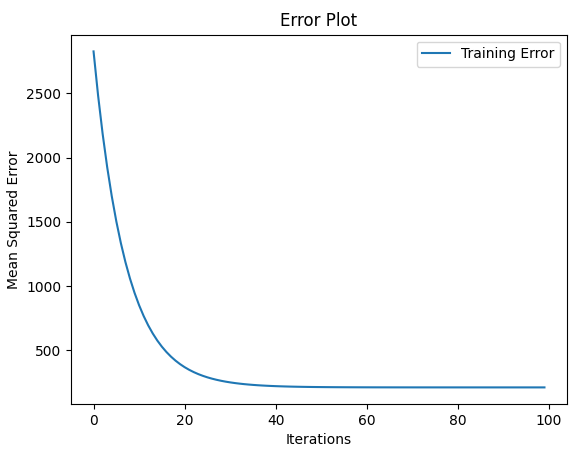
from mlfromscratch.supervised_learning import LinearRegression
 
def main():
 
    X, y = make_regression(n_samples=100, n_features=1, noise=20)
 
    X_train, X_test, y_train, y_test = train_test_split(X, y, test_size=0.4)
 
    n_samples, n_features = np.shape(X)
 
    model = LinearRegression(n_iterations=100)
 
    model.fit(X_train, y_train)
 
    # Training error plot
    n = len(model.training_errors)
    training, = plt.plot(range(n), model.training_errors, label="Training Error")
    plt.legend(handles=[training])
    plt.title("Error Plot")
    plt.ylabel('Mean Squared Error')
    plt.xlabel('Iterations')
    plt.savefig("test1.png")
    plt.show()
 
    y_pred = model.predict(X_test)
    mse = mean_squared_error(y_test, y_pred)
    print ("Mean squared error: %s" % (mse))
 
    y_pred_line = model.predict(X)
 
    # Color map
    cmap = plt.get_cmap('viridis')
 
    # Plot the results
    m1 = plt.scatter(366 * X_train, y_train, color=cmap(0.9), s=10)
    m2 = plt.scatter(366 * X_test, y_test, color=cmap(0.5), s=10)
    plt.plot(366 * X, y_pred_line, color='black', linewidth=2, label="Prediction")
    plt.suptitle("Linear Regression")
    plt.title("MSE: %.2f" % mse, fontsize=10)
    plt.xlabel('Day')
    plt.ylabel('Temperature in Celcius')
    plt.legend((m1, m2), ("Training data", "Test data"), loc='lower right')
    plt.savefig("test2.png")
    plt.show()
 
if __name__ == "__main__":
    main()

利用sklearn库生成线性回归数据，然后将其拆分为训练集和测试集。

utils下的mean_squared_error()：

def mean_squared_error(y_true, y_pred):
    """ Returns the mean squared error between y_true and y_pred """
    mse = np.mean(np.power(y_true - y_pred, 2))
    return mse

结果：

Mean squared error: 532.3321383700828