SSD-tensorflow-1 demo
一、简易识别
用最简单的已训练好的模型对20类目标做检测。
你电脑的tensorflow + CUDA + CUDNN环境都是OK的, 同时python需要安装cv2库
{ 'aeroplane' 'bicycle' 'bird' 'boat' 'bottle' 'bus' 'car' 'cat' 'chair' 'cow' 'diningtable' 'dog' 'horse' 'motorbike' 'person' 'pottedplant' 'sheep' 'sofa' 'train' 'tvmonitor' }
下载好代码后,在checkpoints文件夹下面由ssd_300_vgg.ckpt,直接解压到当前文件夹。
找到notebooks文件夹里的ssd_notebook.ipynb,用jupyter打开。
将读入的图片改为自己的图片就行了(更改path或者将自己的图片放到demo文件夹下面),然后运行所有cells。
- path为你想要进行测试的图片目录(代码中只对该目录下的最后一个文件夹进行测试,如果要想测试多幅图片或者做成视频的方式,需大家自行修改代码)
二、demo2
在notebooks文件夹下,建立demo_test.py文件,在demo_test.py文件内写入如下代码后,直接运行demo_test.py(以下代码也是notebooks文件夹ssd_tests.ipynb内的代码,可以用notebook读取;我只是做了一些小改动)
# -*- coding:utf-8 -*-
# -*- author:zzZ_CMing CSDN address:https://blog.csdn.net/zzZ_CMing
# -*- 2018/07/14; 15:19
# -*- python3.5
"""
address: https://blog.csdn.net/qq_35608277/article/details/78660469
本文代码来自于github中微软官方仓库
"""
import os
import cv2
import math
import random
import tensorflow as tf
import matplotlib.pyplot as plt
import matplotlib.cm as mpcm
import matplotlib.image as mpimg
from notebooks import visualization
from nets import ssd_vgg_300, ssd_common, np_methods
from preprocessing import ssd_vgg_preprocessing
import sys # 当引用模块和运行的脚本不在同一个目录下,需在脚本开头添加如下代码:
sys.path.append('./SSD-Tensorflow/') slim = tf.contrib.slim # TensorFlow session
gpu_options = tf.GPUOptions(allow_growth=True)
config = tf.ConfigProto(log_device_placement=False, gpu_options=gpu_options)
isess = tf.InteractiveSession(config=config) l_VOC_CLASS = ['aeroplane', 'bicycle', 'bird', 'boat', 'bottle',
'bus', 'car', 'cat', 'chair', 'cow',
'diningTable', 'dog', 'horse', 'motorbike', 'person',
'pottedPlant', 'sheep', 'sofa', 'train', 'TV'] # 定义数据格式,设置占位符
net_shape = (300, 300)
# 预处理,以Tensorflow backend, 将输入图片大小改成 300x300,作为下一步输入
img_input = tf.placeholder(tf.uint8, shape=(None, None, 3))
# 输入图像的通道排列形式,'NHWC'表示 [batch_size,height,width,channel]
data_format = 'NHWC' # 数据预处理,将img_input输入的图像resize为300大小,labels_pre,bboxes_pre,bbox_img待解析
image_pre, labels_pre, bboxes_pre, bbox_img = ssd_vgg_preprocessing.preprocess_for_eval(
img_input, None, None, net_shape, data_format,
resize=ssd_vgg_preprocessing.Resize.WARP_RESIZE)
# 拓展为4维变量用于输入
image_4d = tf.expand_dims(image_pre, 0) # 定义SSD模型
# 是否复用,目前我们没有在训练所以为None
reuse = True if 'ssd_net' in locals() else None
# 调出基于VGG神经网络的SSD模型对象,注意这是一个自定义类对象
ssd_net = ssd_vgg_300.SSDNet()
# 得到预测类和预测坐标的Tensor对象,这两个就是神经网络模型的计算流程
with slim.arg_scope(ssd_net.arg_scope(data_format=data_format)):
predictions, localisations, _, _ = ssd_net.net(image_4d, is_training=False, reuse=reuse) # 导入官方给出的 SSD 模型参数
ckpt_filename = '../checkpoints/ssd_300_vgg.ckpt'
# ckpt_filename = '../checkpoints/VGG_VOC0712_SSD_300x300_ft_iter_120000.ckpt'
isess.run(tf.global_variables_initializer())
saver = tf.train.Saver()
saver.restore(isess, ckpt_filename) # 在网络模型结构中,提取搜索网格的位置
# 根据模型超参数,得到每个特征层(这里用了6个特征层,分别是4,7,8,9,10,11)的anchors_boxes
ssd_anchors = ssd_net.anchors(net_shape)
"""
每层的anchors_boxes包含4个arrayList,前两个List分别是该特征层下x,y坐标轴对于原图(300x300)大小的映射
第三,四个List为anchor_box的长度和宽度,同样是经过归一化映射的,根据每个特征层box数量的不同,这两个List元素
个数会变化。其中,长宽的值根据超参数anchor_sizes和anchor_ratios制定。
""" # 加载辅助作图函数
def colors_subselect(colors, num_classes=21):
dt = len(colors) // num_classes
sub_colors = []
for i in range(num_classes):
color = colors[i * dt]
if isinstance(color[0], float):
sub_colors.append([int(c * 255) for c in color])
else:
sub_colors.append([c for c in color])
return sub_colors def bboxes_draw_on_img(img, classes, scores, bboxes, colors, thickness=2):
shape = img.shape
for i in range(bboxes.shape[0]):
bbox = bboxes[i]
color = colors[classes[i]]
# Draw bounding box...
p1 = (int(bbox[0] * shape[0]), int(bbox[1] * shape[1]))
p2 = (int(bbox[2] * shape[0]), int(bbox[3] * shape[1]))
cv2.rectangle(img, p1[::-1], p2[::-1], color, thickness)
# Draw text...
s = '%s/%.3f' % (l_VOC_CLASS[int(classes[i]) - 1], scores[i])
p1 = (p1[0] - 5, p1[1])
# cv2.putText(img, s, p1[::-1], cv2.FONT_HERSHEY_DUPLEX, 1.5, color, 3) colors_plasma = colors_subselect(mpcm.plasma.colors, num_classes=21) # 主流程函数
def process_image(img, case, select_threshold=0.15, nms_threshold=.1, net_shape=(300, 300)):
# select_threshold:box阈值——每个像素的box分类预测数据的得分会与box阈值比较,高于一个box阈值则认为这个box成功框到了一个对象
# nms_threshold:重合度阈值——同一对象的两个框的重合度高于该阈值,则运行下面去重函数 # 执行SSD模型,得到4维输入变量,分类预测,坐标预测,rbbox_img参数为最大检测范围,本文固定为[0,0,1,1]即全图
rimg, rpredictions, rlocalisations, rbbox_img = isess.run([image_4d, predictions,
localisations, bbox_img], feed_dict={img_input: img}) # ssd_bboxes_select()函数根据每个特征层的分类预测分数,归一化后的映射坐标,
# ancohor_box的大小,通过设定一个阈值计算得到每个特征层检测到的对象以及其分类和坐标
rclasses, rscores, rbboxes = np_methods.ssd_bboxes_select(rpredictions, rlocalisations, ssd_anchors,
select_threshold=select_threshold,
img_shape=net_shape,
num_classes=21, decode=True) """
这个函数做的事情比较多,这里说的细致一些:
首先是输入,输入的数据为每个特征层(一共6个,见上文)的:
rpredictions: 分类预测数据,
rlocalisations: 坐标预测数据,
ssd_anchors: anchors_box数据
其中:
分类预测数据为当前特征层中每个像素的每个box的分类预测
坐标预测数据为当前特征层中每个像素的每个box的坐标预测
anchors_box数据为当前特征层中每个像素的每个box的修正数据 函数根据坐标预测数据和anchors_box数据,计算得到每个像素的每个box的中心和长宽,这个中心坐标和长宽会根据一个算法进行些许的修正,
从而得到一个更加准确的box坐标;修正的算法会在后文中详细解释,如果只是为了理解算法流程也可以不必深究这个,因为这个修正算法属于经验算
法,并没有太多逻辑可循。
修正完box和中心后,函数会计算每个像素的每个box的分类预测数据的得分,当这个分数高于一个阈值(这里是0.5)则认为这个box成功
框到了一个对象,然后将这个box的坐标数据,所属分类和分类得分导出,从而得到:
rclasses:所属分类
rscores:分类得分
rbboxes:坐标 最后要注意的是,同一个目标可能会在不同的特征层都被检测到,并且他们的box坐标会有些许不同,这里并没有去掉重复的目标,而是在下文
中专门用了一个函数来去重
""" # 检测有没有超出检测边缘
rbboxes = np_methods.bboxes_clip(rbbox_img, rbboxes)
rclasses, rscores, rbboxes = np_methods.bboxes_sort(rclasses, rscores, rbboxes, top_k=400)
# 去重,将重复检测到的目标去掉
rclasses, rscores, rbboxes = np_methods.bboxes_nms(rclasses, rscores, rbboxes, nms_threshold=nms_threshold)
# 将box的坐标重新映射到原图上(上文所有的坐标都进行了归一化,所以要逆操作一次)
rbboxes = np_methods.bboxes_resize(rbbox_img, rbboxes) if case == 1:
bboxes_draw_on_img(img, rclasses, rscores, rbboxes, colors_plasma, thickness=8)
return img
else:
return rclasses, rscores, rbboxes """
# 只做目标定位,不做预测分析
case = 1
img = cv2.imread("../demo/person.jpg")
img = cv2.cvtColor(img, cv2.COLOR_BGR2RGB)
plt.imshow(process_image(img, case))
plt.show()
"""
# 做目标定位,同时做预测分析
case = 2
path = '../demo/person.jpg'
# 读取图片
img = mpimg.imread(path)
# 执行主流程函数
rclasses, rscores, rbboxes = process_image(img, case)
# visualization.bboxes_draw_on_img(img, rclasses, rscores, rbboxes, visualization.colors_plasma)
# 显示分类结果图
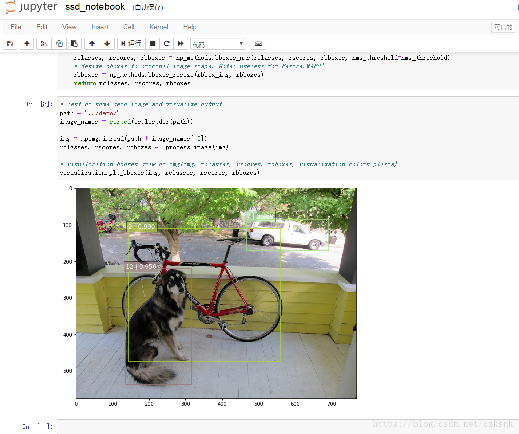
visualization.plt_bboxes(img, rclasses, rscores, rbboxes), rscores, rbboxes
会得到如下图示,如图已经成功的把物体标注出来,每个标记框中前一个数是标签项,后一个是预测的准确率;
# 标签项与其对应的标签内容
dict = {1:'aeroplane', 2:'bicycle', 3:'bird', 4:'boat', 5:'bottle',
6:'bus', 7:'car', 8:'cat', 9:'chair', 10:'cow',
11:'diningTable', 12:'dog', 13:'horse', 14:'motorbike', 15:'person',
16:'pottedPlant', 17:'sheep', 18:'sofa', 19:'train', 20:'TV'}

三、demo3 视频定位检测
以上demo文件夹内都只是图片,如果你想在视频中标记物体——首先你需要拍一段视频,建议不要太长不然你要跑很久,然后需要在主目录下建立Video文件夹,在其下建立input、output文件夹,如下图所示:
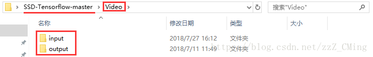
再将拍摄的视频存入input文件夹下,注意视频的名称哦!最后在主目录下建立demo_Video.py文件,存入如下代码,运行demo_Video.py
请注意:166行的文件名要与文件夹视频名一致
请注意:166行的文件名要与文件夹视频名一致
 # -*- coding:utf-8 -*-

 # -*- author:zzZ_CMing  CSDN address:https://blog.csdn.net/zzZ_CMing

 # -*- 2018/07/09; 15:19

 # -*- python3.5

 import os

 import cv2

 import math

 import random

 import tensorflow as tf

 import matplotlib.pyplot as plt

 import matplotlib.cm as mpcm

 import matplotlib.image as mpimg

 from notebooks import visualization

 from nets import ssd_vgg_300, ssd_common, np_methods

 from preprocessing import ssd_vgg_preprocessing

 import sys

 # 当引用模块和运行的脚本不在同一个目录下,需在脚本开头添加如下代码:

 sys.path.append('./SSD-Tensorflow/')

 slim = tf.contrib.slim

 # TensorFlow session

 gpu_options = tf.GPUOptions(allow_growth=True)

 config = tf.ConfigProto(log_device_placement=False, gpu_options=gpu_options)

 isess = tf.InteractiveSession(config=config)

 l_VOC_CLASS = ['aeroplane', 'bicycle', 'bird', 'boat', 'bottle',

                'bus', 'car', 'cat', 'chair', 'cow',

                'diningTable', 'dog', 'horse', 'motorbike', 'person',

                'pottedPlant', 'sheep', 'sofa', 'train', 'TV']

 # 定义数据格式,设置占位符

 net_shape = (300, 300)

 # 预处理,以Tensorflow backend, 将输入图片大小改成 300x300,作为下一步输入

 img_input = tf.placeholder(tf.uint8, shape=(None, None, 3))

 # 输入图像的通道排列形式,'NHWC'表示 [batch_size,height,width,channel]

 data_format = 'NHWC'

 # 数据预处理,将img_input输入的图像resize为300大小,labels_pre,bboxes_pre,bbox_img待解析

 image_pre, labels_pre, bboxes_pre, bbox_img = ssd_vgg_preprocessing.preprocess_for_eval(

     img_input, None, None, net_shape, data_format,

     resize=ssd_vgg_preprocessing.Resize.WARP_RESIZE)

 # 拓展为4维变量用于输入

 image_4d = tf.expand_dims(image_pre, 0)

 # 定义SSD模型

 # 是否复用,目前我们没有在训练所以为None

 reuse = True if 'ssd_net' in locals() else None

 # 调出基于VGG神经网络的SSD模型对象,注意这是一个自定义类对象

 ssd_net = ssd_vgg_300.SSDNet()

 # 得到预测类和预测坐标的Tensor对象,这两个就是神经网络模型的计算流程

 with slim.arg_scope(ssd_net.arg_scope(data_format=data_format)):

     predictions, localisations, _, _ = ssd_net.net(image_4d, is_training=False, reuse=reuse)

 # 导入官方给出的 SSD 模型参数

 ckpt_filename = '../checkpoints/ssd_300_vgg.ckpt'

 # ckpt_filename = '../checkpoints/VGG_VOC0712_SSD_300x300_ft_iter_120000.ckpt'

 isess.run(tf.global_variables_initializer())

 saver = tf.train.Saver()

 saver.restore(isess, ckpt_filename)

 # 在网络模型结构中,提取搜索网格的位置

 # 根据模型超参数,得到每个特征层(这里用了6个特征层,分别是4,7,8,9,10,11)的anchors_boxes

 ssd_anchors = ssd_net.anchors(net_shape)

 """

 每层的anchors_boxes包含4个arrayList,前两个List分别是该特征层下x,y坐标轴对于原图(300x300)大小的映射

 第三,四个List为anchor_box的长度和宽度,同样是经过归一化映射的,根据每个特征层box数量的不同,这两个List元素

 个数会变化。其中,长宽的值根据超参数anchor_sizes和anchor_ratios制定。

 """

 # 加载辅助作图函数

 def colors_subselect(colors, num_classes=21):

     dt = len(colors) // num_classes

     sub_colors = []

     for i in range(num_classes):

         color = colors[i * dt]

         if isinstance(color[0], float):

             sub_colors.append([int(c * 255) for c in color])

         else:

             sub_colors.append([c for c in color])

     return sub_colors

 def bboxes_draw_on_img(img, classes, scores, bboxes, colors, thickness=2):

     shape = img.shape

     for i in range(bboxes.shape[0]):

         bbox = bboxes[i]

         color = colors[classes[i]]

         # Draw bounding box...

         p1 = (int(bbox[0] * shape[0]), int(bbox[1] * shape[1]))

         p2 = (int(bbox[2] * shape[0]), int(bbox[3] * shape[1]))

         cv2.rectangle(img, p1[::-1], p2[::-1], color, thickness)

         # Draw text...

         s = '%s/%.3f' % (l_VOC_CLASS[int(classes[i]) - 1], scores[i])

         p1 = (p1[0] - 5, p1[1])

         # cv2.putText(img, s, p1[::-1], cv2.FONT_HERSHEY_DUPLEX, 1.5, color, 3)

 colors_plasma = colors_subselect(mpcm.plasma.colors, num_classes=21)

 # 主流程函数

 def process_image(img, select_threshold=0.2, nms_threshold=.1, net_shape=(300, 300)):

     # select_threshold:box阈值——每个像素的box分类预测数据的得分会与box阈值比较,高于一个box阈值则认为这个box成功框到了一个对象

     # nms_threshold:重合度阈值——同一对象的两个框的重合度高于该阈值,则运行下面去重函数

     # 执行SSD模型,得到4维输入变量,分类预测,坐标预测,rbbox_img参数为最大检测范围,本文固定为[0,0,1,1]即全图

     rimg, rpredictions, rlocalisations, rbbox_img = isess.run([image_4d, predictions, localisations, bbox_img],

                                                               feed_dict={img_input: img})

     # ssd_bboxes_select函数根据每个特征层的分类预测分数,归一化后的映射坐标,

     # ancohor_box的大小,通过设定一个阈值计算得到每个特征层检测到的对象以及其分类和坐标

     rclasses, rscores, rbboxes = np_methods.ssd_bboxes_select(rpredictions, rlocalisations, ssd_anchors,

                                                               select_threshold=select_threshold,

                                                               img_shape=net_shape,

                                                               num_classes=21, decode=True)

     """

     这个函数做的事情比较多,这里说的细致一些:

     首先是输入,输入的数据为每个特征层(一共6个,见上文)的:

                                                 分类预测数据(rpredictions),

                                                 坐标预测数据(rlocalisations),

                                                 anchors_box数据(ssd_anchors)

                                             其中:

                                                分类预测数据为当前特征层中每个像素的每个box的分类预测

                                                坐标预测数据为当前特征层中每个像素的每个box的坐标预测

                                                anchors_box数据为当前特征层中每个像素的每个box的修正数据

         函数根据坐标预测数据和anchors_box数据,计算得到每个像素的每个box的中心和长宽,这个中心坐标和长宽会根据一个算法进行些许的修正,

     从而得到一个更加准确的box坐标;修正的算法会在后文中详细解释,如果只是为了理解算法流程也可以不必深究这个,因为这个修正算法属于经验算

     法,并没有太多逻辑可循。

         修正完box和中心后,函数会计算每个像素的每个box的分类预测数据的得分,当这个分数高于一个阈值(这里是0.5)则认为这个box成功

     框到了一个对象,然后将这个box的坐标数据,所属分类和分类得分导出,从而得到:

         rclasses:所属分类

         rscores:分类得分

         rbboxes:坐标

         最后要注意的是,同一个目标可能会在不同的特征层都被检测到,并且他们的box坐标会有些许不同,这里并没有去掉重复的目标,而是在下文

     中专门用了一个函数来去重

     """

     # 检测有没有超出检测边缘

     rbboxes = np_methods.bboxes_clip(rbbox_img, rbboxes)

     rclasses, rscores, rbboxes = np_methods.bboxes_sort(rclasses, rscores, rbboxes, top_k=400)

     # 去重,将重复检测到的目标去掉

     rclasses, rscores, rbboxes = np_methods.bboxes_nms(rclasses, rscores, rbboxes, nms_threshold=nms_threshold)

     # 将box的坐标重新映射到原图上(上文所有的坐标都进行了归一化,所以要逆操作一次)

     rbboxes = np_methods.bboxes_resize(rbbox_img, rbboxes)

     bboxes_draw_on_img(img, rclasses, rscores, rbboxes, colors_plasma, thickness=8)

     return img

 # 视频物体定位

 import imageio

 imageio.plugins.ffmpeg.download()

 from moviepy.editor import VideoFileClip

 def process_video (input_path, output_path):

     video = VideoFileClip(input_path)

     result = video.fl_image(process_image)

     result.write_videofile(output_path, fps=40)

 video_name = "3.mp4"

 input_path = "./Video/input/" + video_name

 output_path = "./Video/output/output_" + video_name

 process_video(input_path,output_path )
经过一段时间的等待,终于跑完程序;
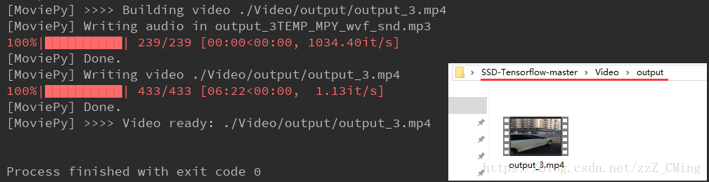
打开Video/input文件夹,查看输出的视频是什么样子的吧!
四、demo4-视频(显示标签)
notebook目录下新建ssd_notebook_camera.py:
# coding: utf-8

import os

import math

import random

import numpy as np

import tensorflow as tf

import cv2

slim = tf.contrib.slim

# get_ipython().magic('matplotlib inline')

import matplotlib.pyplot as plt

import matplotlib.image as mpimg

import sys

sys.path.append('../')

from nets import ssd_vgg_300, ssd_common, np_methods

from preprocessing import ssd_vgg_preprocessing

from notebooks import visualization_camera  # visualization

# TensorFlow session: grow memory when needed. TF, DO NOT USE ALL MY GPU MEMORY!!!

gpu_options = tf.GPUOptions(allow_growth=True)

config = tf.ConfigProto(log_device_placement=False, gpu_options=gpu_options)

isess = tf.InteractiveSession(config=config)

# ## SSD 300 Model

#

# The SSD 300 network takes 300x300 image inputs. In order to feed any image, the latter is resize to this input shape (i.e.`Resize.WARP_RESIZE`). Note that even though it may change the ratio width / height, the SSD model performs well on resized images (and it is the default behaviour in the original Caffe implementation).

#

# SSD anchors correspond to the default bounding boxes encoded in the network. The SSD net output provides offset on the coordinates and dimensions of these anchors.

# Input placeholder.

net_shape = (300, 300)

data_format = 'NHWC'

img_input = tf.placeholder(tf.uint8, shape=(None, None, 3))

# Evaluation pre-processing: resize to SSD net shape.

image_pre, labels_pre, bboxes_pre, bbox_img = ssd_vgg_preprocessing.preprocess_for_eval(

    img_input, None, None, net_shape, data_format, resize=ssd_vgg_preprocessing.Resize.WARP_RESIZE)

image_4d = tf.expand_dims(image_pre, 0)

# Define the SSD model.

reuse = True if 'ssd_net' in locals() else None

ssd_net = ssd_vgg_300.SSDNet()

with slim.arg_scope(ssd_net.arg_scope(data_format=data_format)):

    predictions, localisations, _, _ = ssd_net.net(image_4d, is_training=False, reuse=reuse)

# Restore SSD model.

ckpt_filename = 'E:/SSD/initial_SSD/SSD-Tensorflow-master/checkpoints/ssd_300_vgg.ckpt'  # 可更改为自己的模型路径

# ckpt_filename = '../checkpoints/VGG_VOC0712_SSD_300x300_ft_iter_120000.ckpt'

isess.run(tf.global_variables_initializer())

saver = tf.train.Saver()

saver.restore(isess, ckpt_filename)

# SSD default anchor boxes.

ssd_anchors = ssd_net.anchors(net_shape)

# ## Post-processing pipeline

#

# The SSD outputs need to be post-processed to provide proper detections. Namely, we follow these common steps:

#

# * Select boxes above a classification threshold;

# * Clip boxes to the image shape;

# * Apply the Non-Maximum-Selection algorithm: fuse together boxes whose Jaccard score > threshold;

# * If necessary, resize bounding boxes to original image shape.

# Main image processing routine.

def process_image(img, select_threshold=0.5, nms_threshold=.45, net_shape=(300, 300)):

    # Run SSD network.

    rimg, rpredictions, rlocalisations, rbbox_img = isess.run([image_4d, predictions, localisations, bbox_img],

                                                              feed_dict={img_input: img})

    # Get classes and bboxes from the net outputs.

    rclasses, rscores, rbboxes = np_methods.ssd_bboxes_select(

        rpredictions, rlocalisations, ssd_anchors,

        select_threshold=select_threshold, img_shape=net_shape, num_classes=21, decode=True)

    rbboxes = np_methods.bboxes_clip(rbbox_img, rbboxes)

    rclasses, rscores, rbboxes = np_methods.bboxes_sort(rclasses, rscores, rbboxes, top_k=400)

    rclasses, rscores, rbboxes = np_methods.bboxes_nms(rclasses, rscores, rbboxes, nms_threshold=nms_threshold)

    # Resize bboxes to original image shape. Note: useless for Resize.WARP!

    rbboxes = np_methods.bboxes_resize(rbbox_img, rbboxes)

    return rclasses, rscores, rbboxes

# # Test on some demo image and visualize output.

# path = '../demo/'

# image_names = sorted(os.listdir(path))

# img = mpimg.imread(path + image_names[-5])

# rclasses, rscores, rbboxes =  process_image(img)

# # visualization.bboxes_draw_on_img(img, rclasses, rscores, rbboxes, visualization.colors_plasma)

# visualization.plt_bboxes(img, rclasses, rscores, rbboxes)

##### following are added for camera demo####

cap = cv2.VideoCapture(r'E:/SSD/initial_SSD/SSD-Tensorflow-master/demo_video/01.mp4')

fps = cap.get(cv2.CAP_PROP_FPS)

size = (int(cap.get(cv2.CAP_PROP_FRAME_WIDTH)), int(cap.get(cv2.CAP_PROP_FRAME_HEIGHT)))

fourcc = cap.get(cv2.CAP_PROP_FOURCC)

# fourcc = cv2.CAP_PROP_FOURCC(*'CVID')

print('fps=%d,size=%r,fourcc=%r' % (fps, size, fourcc))

delay = 30 / int(fps)

while (cap.isOpened()):

    ret, frame = cap.read()

    if ret == True:

        #          image = Image.open(image_path)

        #          gray = cv2.cvtColor(frame, cv2.COLOR_BGR2GRAY)

        image = frame

        # the array based representation of the image will be used later in order to prepare the

        # result image with boxes and labels on it.

        image_np = image

        #          image_np = load_image_into_numpy_array(image)

        # Expand dimensions since the model expects images to have shape: [1, None, None, 3]

        image_np_expanded = np.expand_dims(image_np, axis=0)

        # Actual detection.

        rclasses, rscores, rbboxes = process_image(image_np)

        # Visualization of the results of a detection.

        visualization_camera.bboxes_draw_on_img(image_np, rclasses, rscores, rbboxes)

        #          plt.figure(figsize=IMAGE_SIZE)

        #          plt.imshow(image_np)

        cv2.imshow('frame', image_np)

        cv2.waitKey(np.uint(delay))

        print('Ongoing...')

    else:

        break

cap.release()

cv2.destroyAllWindows()
此外还要新建visualization.py:
 # Copyright 2017 Paul Balanca. All Rights Reserved.

 #

 # Licensed under the Apache License, Version 2.0 (the "License");

 # you may not use this file except in compliance with the License.

 # You may obtain a copy of the License at

 #

 #     http://www.apache.org/licenses/LICENSE-2.0

 #

 # Unless required by applicable law or agreed to in writing, software

 # distributed under the License is distributed on an "AS IS" BASIS,

 # WITHOUT WARRANTIES OR CONDITIONS OF ANY KIND, either express or implied.

 # See the License for the specific language governing permissions and

 # limitations under the License.

 # ==============================================================================

 import cv2

 import random

 import matplotlib.pyplot as plt

 import matplotlib.image as mpimg

 import matplotlib.cm as mpcm

 #这是一个mixin类,用于支持标量数据到RGBA映射。ScalarMappable在从给定的colormap返回RGBA颜色之前使用数据规范化。

 def num2class(n):

     import datasets.pascalvoc_2007 as pas

     x = pas.pascalvoc_common.VOC_LABELS.items()

     for name, item in x:

         if n in item:

             # print(name)

             return name

 # =========================================================================== #

 # Some colormaps.

 # =========================================================================== #

 def colors_subselect(colors, num_classes=21):

     dt = len(colors) // num_classes

     sub_colors = []

     for i in range(num_classes):

         color = colors[i * dt]

         if isinstance(color[0], float):

             sub_colors.append([int(c * 255) for c in color])

         else:

             sub_colors.append([c for c in color])

     return sub_colors

 colors_plasma = colors_subselect(mpcm.plasma.colors, num_classes=21)

 colors_tableau = [(255, 255, 255), (31, 119, 180), (174, 199, 232), (255, 127, 14), (255, 187, 120),

                   (44, 160, 44), (152, 223, 138), (214, 39, 40), (255, 152, 150),

                   (148, 103, 189), (197, 176, 213), (140, 86, 75), (196, 156, 148),

                   (227, 119, 194), (247, 182, 210), (127, 127, 127), (199, 199, 199),

                   (188, 189, 34), (219, 219, 141), (23, 190, 207), (158, 218, 229)]

 # =========================================================================== #

 # OpenCV drawing.

 # =========================================================================== #

 def draw_lines(img, lines, color=[255, 0, 0], thickness=2):

     """Draw a collection of lines on an image.

     """

     for line in lines:

         for x1, y1, x2, y2 in line:

             cv2.line(img, (x1, y1), (x2, y2), color, thickness)

 def draw_rectangle(img, p1, p2, color=[255, 0, 0], thickness=2):

     cv2.rectangle(img, p1[::-1], p2[::-1], color, thickness)

 def draw_bbox(img, bbox, shape, label, color=[255, 0, 0], thickness=2):

     p1 = (int(bbox[0] * shape[0]), int(bbox[1] * shape[1]))

     p2 = (int(bbox[2] * shape[0]), int(bbox[3] * shape[1]))

     cv2.rectangle(img, p1[::-1], p2[::-1], color, thickness)

     p1 = (p1[0] + 15, p1[1])

     cv2.putText(img, str(label), p1[::-1], cv2.FONT_HERSHEY_DUPLEX, 0.5, color, 1)

 def bboxes_draw_on_img(img, classes, scores, bboxes, colors=dict(), thickness=2):

     shape = img.shape

     ####add 20180516#####

     # colors=dict()

     ####add #############

     for i in range(bboxes.shape[0]):

         bbox = bboxes[i]

         if classes[i] not in colors:

             colors[classes[i]] = (random.random(), random.random(), random.random())

         p1 = (int(bbox[0] * shape[0]), int(bbox[1] * shape[1]))

         p2 = (int(bbox[2] * shape[0]), int(bbox[3] * shape[1]))

         cv2.rectangle(img, p1[::-1], p2[::-1], colors[classes[i]], thickness)

         s = '%s/%.3f' % (num2class(classes[i]), scores[i])

         p1 = (p1[0] - 5, p1[1])

         cv2.putText(img, s, p1[::-1], cv2.FONT_HERSHEY_DUPLEX, 0.4, colors[classes[i]], 1)

     # =========================================================================== #

 # Matplotlib show...

 # =========================================================================== #

 def plt_bboxes(img, classes, scores, bboxes, figsize=(10, 10), linewidth=1.5):

     """Visualize bounding boxes. Largely inspired by SSD-MXNET!

     """

     fig = plt.figure(figsize=figsize)

     plt.imshow(img)

     height = img.shape[0]

     width = img.shape[1]

     colors = dict()

     for i in range(classes.shape[0]):

         cls_id = int(classes[i])

         if cls_id >= 0:

             score = scores[i]

             if cls_id not in colors:

                 colors[cls_id] = (random.random(), random.random(), random.random())

             ymin = int(bboxes[i, 0] * height)

             xmin = int(bboxes[i, 1] * width)

             ymax = int(bboxes[i, 2] * height)

             xmax = int(bboxes[i, 3] * width)

             rect = plt.Rectangle((xmin, ymin), xmax - xmin,

                                  ymax - ymin, fill=False,

                                  edgecolor=colors[cls_id],

                                  linewidth=linewidth)

             plt.gca().add_patch(rect)

             ##class_name = str(cls_id) #commented 20180516

             #### added 20180516#####

             class_name = num2class(cls_id)

             #### added end #########

             plt.gca().text(xmin, ymin - 2,

                            '{:s} | {:.3f}'.format(class_name, score),

                            bbox=dict(facecolor=colors[cls_id], alpha=0.5),

                            fontsize=12, color='white')

     plt.show()
SSD-tensorflow-1 demo的更多相关文章
- TensorFlow Lite demo——就是为嵌入式设备而存在的,底层调用NDK神经网络API,注意其使用的tf model需要转换下,同时提供java和C++ API,无法使用tflite的见后
Introduction to TensorFlow Lite TensorFlow Lite is TensorFlow’s lightweight solution for mobile and ...
- 【目标检测】SSD+Tensorflow 300&512 配置详解
SSD_300_vgg和SSD_512_vgg weights下载链接[需要科学上网~]: Model Training data Testing data mAP FPS SSD-300 VGG-b ...
- Ubuntu 使用 Android Studio 编译 TensorFlow android demo
https://www.cnblogs.com/dyufei/p/8028218.html https://www.myboxlab.com/topic/detail/714ca2d405414f13 ...
- tensorflow summary demo with linear-model
tf.summary + tensorboard 用来把graph图中的相关信息,如结构图.学习率.准确率.Loss等数据,写入到本地硬盘,并通过浏览器可视化之. 整理的代码如下: import te ...
- Ubuntu18.04使用AndroidStudio3.2.1编译TensorFlow android demo【2018年12月】
按照官方教程修改下面3处即可编译完成. 修改部分: 在build.gradle文件里修改以下部分: 1.原来: buildscript { repositories { jcenter() } dep ...
- SSD:TensorFlow中的单次多重检测器
SSD:TensorFlow中的单次多重检测器 SSD Notebook 包含 SSD TensorFlow 的最小示例. 很快,就检测出了两个主要步骤:在图像上运行SSD网络,并使用通用算法(top ...
- android应用市场、社区客户端、漫画App、TensorFlow Demo、歌词显示、动画效果等源码
Android精选源码 MVP架构Android应用市场项目 android刻度盘控件源码 Android实现一个社区客户端 android商品详情页上拉查看详情 基于RxJava+Retrofit2 ...
- 论文笔记 SSD: Single Shot MultiBox Detector
转载自:https://zhuanlan.zhihu.com/p/33544892 前言 目标检测近年来已经取得了很重要的进展,主流的算法主要分为两个类型(参考RefineDet):(1)two-st ...
- tensorflow入门(1):构造线性回归模型
今天让我们一起来学习如何用TF实现线性回归模型.所谓线性回归模型就是y = W * x + b的形式的表达式拟合的模型. 我们先假设一条直线为 y = 0.1x + 0.3,即W = 0.1,b = ...
- TensorFlow 生成 .ckpt 和 .pb
原文:https://www.cnblogs.com/nowornever-L/p/6991295.html 1. TensorFlow 生成的 .ckpt 和 .pb 都有什么用? The . ...
随机推荐
- Under ubuntu 12.04,install sublime text 2
Sublime Text is an awesome text editor. If you’ve never heard of it, you should check it out right n ...
- requireJS实现原理分析
下面requireJS实现的基本思路 项目地址https://github.com/WangMaoling/require var require = (function(){ //框架版本基本信息 ...
- 你不知道的JavaScript(十)with关键字
with关键字在JavaScript中不太常用,用来定义一个和对象相关的作用域,在该作用域中可以访问对象的属性或方法而前面无需加上对象名,以达到简化代码的目的. <script type=&qu ...
- Servlet学习(七)——cookie
一.会话技术简介 1.存储客户端的状态 例如网站的购物系统,用户将购买的商品信息存储到哪里?因为Http协议是无状态的,也就是说每个客户访问服务器端资源时,服务器并不知道该客户端是谁,所以需要会话技术 ...
- windows下安装mycat,并简单使用
使用mycat需要先安装jdk1.7以上 参考:http://www.cnblogs.com/llhhll/p/9257764.html 1从官网下载解压后目录如下(1.6版本) 下载地址:https ...
- 记一次使用 removeEventListener 移除事件监听失败的经历
测试一 测试代码如下 var Test = function() { this.element = document.body; this.handler = function() { console ...
- hiho160周 - 字符串压缩,经典dp
题目链接 小Hi希望压缩一个只包含大写字母'A'-'Z'的字符串.他使用的方法是:如果某个子串 S 连续出现了 X 次,就用'X(S)'来表示.例如AAAAAAAAAABABABCCD可以用10(A) ...
- git远程仓库变更
查看自己的远程仓库 git remote -v 远程仓库变更 git remote remove origin //移出现有的远程仓库的地址 git remote add origin http:// ...
- 强化学习(3)-----DQN
看这篇https://blog.csdn.net/qq_16234613/article/details/80268564 1.DQN 原因:在普通的Q-learning中,当状态和动作空间是离散且维 ...
- redis.conf配置文件配置项解析
知识来源于 : https://blog.csdn.net/bsfz_2018/article/details/79061413[Redis在linux下的安装] daemonize:如需要在后台运行 ...