7 Recursive AutoEncoder结构递归自编码器(tensorflow)不能调用GPU进行计算的问题（非机器配置，而是网络结构的问题）

一、源代码下载

代码最初来源于Github：https://github.com/vijayvee/Recursive-neural-networks-TensorFlow，代码介绍如下：“This repository contains the implementation of a single hidden layer Recursive Neural Network.Implemented in python using TensorFlow. Used the trained models for the task of Positive/Negative sentiment analysis. This code is the solution for the third programming assignment from "CS224d: Deep learning for Natural Language Processing", Stanford University.”

由于其运行在python2版本，我对其进行了修改，以及对相关树进行了可视化。我修改后的可运行代码下载链接是（连同要处理的电影评论数据）：

https://pan.baidu.com/s/1bJTulQPs_h25sdLlCcTqDA

运行环境是：windows10、anaconda上创建的tensorflow1.8环境、python3.6版本。

二、问题描述

在程序中使用log_device_placement=True，可以看到：

运算设备的选择是GPU，只有部分save/restore操作是CPU。

但是实际运行的时候，GPU Load为0。

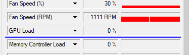
我的电脑已经是GPU安装完整的，运行其它的神经网络程序，能够看到GPU Load的变化。

三、解决方案

提交到付费解决方案平台昂钛客https://www.angtk.com/

https://www.angtk.com/question/354

没有收到问题的解决办法。

四、部分发现

第一，RvNN网络是随着语料库中的句子（训练样本）长度的变化而变化。

第二，由于第一方面的特性，其必须设定一个reset_after。即每训练reset_after个句子，就需要保存模型，接着重新定义一个新的Graph，然后将已经保存模型中的

权值矩阵恢复到新的Graph中，继续进行训练。

我在我修改的代码中加入了保存计算图的操作，可以用tensorboard查看。观察发现，每训练reset_after个句子，就会生成reset_after个loss层（每个句子对应一个loss层），计算图会越来越大。

这也是为什么要重新定义Graph，然后继续训练。

（结构递归神经网络RvNN的核心就是一个前向层和一个重构层，这两个层不断应用于两个子节点，然后得出父节点。所以，这两个层的参数是被不断训练的）

五、解决方案

5.1：收集其它RvNN的实现

大部分的实现都是Richard Socher写的Matlab程序以及对应的Python版本，都包括了损失值的计算和梯度值的计算。我需要找到的是tensorflow版本上的实现。

参考网址：https://stats.stackexchange.com/questions/243221/recursive-neural-network-implementation-in-tensorflow里面提供了一些实现的方法

5.1.1  TensorFlow Fold

https://github.com/tensorflow/fold

TensorFlow Fold is a library for creating TensorFlow models that consume structured data, where the structure of the computation graph depends on the structure of the input data. For example, this model implements TreeLSTMs for sentiment analysis on parse trees of arbitrary shape/size/depth.

Fold implements dynamic batching. Batches of arbitrarily shaped computation graphs are transformed to produce a static computation graph. This graph has the same structure regardless of what input it receives, and can be executed efficiently by TensorFlow.

This animation shows a recursive neural network run with dynamic batching. Operations of the same type appearing at the same depth in the computation graph (indicated by color in the animiation) are batched together regardless of whether or not they appear in the same parse tree. The Embed operation converts words to vector representations. The fully connected (FC) operation combines word vectors to form vector representations of phrases. The output of the network is a vector representation of an entire sentence. Although only a single parse tree of a sentence is shown, the same network can run, and batch together operations, over multiple parse trees of arbitrary shapes and sizes. The TensorFlow concat, while_loop, and gather ops are created once, prior to variable initialization, by Loom, the low-level API for TensorFlow Fold.

(里面提到了三个运算，concat，while和gather)

5.1.2 Tensorflow implementation of Recursive Neural Networks using LSTM units

下载地址是：https://github.com/sapruash/RecursiveNN

Tensorflow implementation of Recursive Neural Networks using LSTM units as described in "Improved Semantic Representations From Tree-Structured Long Short-Term Memory Networks" by Kai Sheng Tai, Richard Socher, and Christopher D. Manning.

（这个是斯坦福Richard Socher教授的文章，他是RvNN的提出者，他在博士论文中阐述了这个网络结构，也因此成为了深度学习大神之一）

5.1.3 Recursive (not Recurrent!) Neural Networks in TensorFlow

（KDnuggets）

文章地址：https://www.kdnuggets.com/2016/06/recursive-neural-networks-tensorflow.html

代码下载地址（需要翻墙）：https://gist.github.com/anj1/504768e05fda49a6e3338e798ae1cddd

我简单的从py2转到py3上以后，运行，发现Gpu load已经上来了，不再是0.

所以，我怀疑本文没有调用GPU的代码是因为网络结构定义中使用了dict的缘故。在字典中放入tensor向量，导致不被GPU运算支持。现在我对代码进行重构。

---

RvNN的两个缺点

The advantage of TreeNets is that they can be very powerful in learning hierarchical, tree-like structure. The disadvantages are, firstly, that the tree structure of every input sample must be known at training time. We will represent the tree structure like this (lisp-like notation):

(S (NP that movie) (VP was) (ADJP cool))

In each sub-expression, the type of the sub-expression must be given – in this case, we are parsing a sentence, and the type of the sub-expression is simply the part-of-speech (POS) tag. You can see that expressions with three elements (one head and two tail elements) correspond to binary operations, whereas those with four elements (one head and three tail elements) correspond to trinary operations, etc.

The second disadvantage of TreeNets is that training is hard because the tree structure changes for each training sample and it’s not easy to map training to mini-batches and so on.

6 调试解决问题。

6.1 调试Recursive (not Recurrent!) Neural Networks in TensorFlow

源代码

import types
import tensorflow as tf
import numpy as np
 
# Expressions are represented as lists of lists,
# in lisp style -- the symbol name is the head (first element)
# of the list, and the arguments follow.
 
# add an expression to an expression list, recursively if necessary.
def add_expr_to_list(exprlist, expr):
    # if expr is a atomic type
    if isinstance(expr, list):
        # Now for rest of expression
        for e in expr[1:]:
            # Add to list if necessary
            if not (e in exprlist):
                add_expr_to_list(exprlist, e)
    # Add index in list.
    exprlist.append(expr)
 
def expand_subexprs(exprlist):
    new_exprlist = []
    orig_indices = []
    for e in exprlist:
        add_expr_to_list(new_exprlist, e)
        orig_indices.append(len(new_exprlist)-1)
    return new_exprlist, orig_indices
 
def compile_expr(exprlist, expr):
    # start new list starting with head
    new_expr = [expr[0]]
    for e in expr[1:]:
        new_expr.append(exprlist.index(e))
    return new_expr
 
def compile_expr_list(exprlist):
    new_exprlist = []
    for e in exprlist:
        if isinstance(e, list):
            new_expr = compile_expr(exprlist, e)
        else:
            new_expr = e
        new_exprlist.append(new_expr)
    return new_exprlist
 
def expand_and_compile(exprlist):
    l, orig_indices = expand_subexprs(exprlist)
    return compile_expr_list(l), orig_indices
 
def new_weight(N1,N2):
    return tf.Variable(tf.random_normal([N1,N2]))
def new_bias(N_hidden):
    return tf.Variable(tf.random_normal([N_hidden]))
 
def build_weights(exprlist,N_hidden,inp_vec_len,out_vec_len):
    W = dict()  # dict of weights corresponding to each operation
    b = dict()  # dict of biases corresponding to each operation
    W['input']  = new_weight(inp_vec_len, N_hidden)
    W['output'] = new_weight(N_hidden, out_vec_len)
    for expr in exprlist:
        if isinstance(expr, list):
            idx = expr[0]
            if not (idx in W):
                W[idx] = [new_weight(N_hidden,N_hidden) for i in expr[1:]]
                b[idx] = new_bias(N_hidden)
    return (W,b)
 
def build_rnn_graph(exprlist,W,b,inp_vec_len):
    # with W built up, create list of variables
    # intermediate variables
    in_vars = [e for e in exprlist if not isinstance(e,list)]
    N_input = len(in_vars)
    inp_tensor = tf.placeholder(tf.float32, (N_input,  inp_vec_len), name='input1')
    V = []      # list of variables corresponding to each expr in exprlist
    for expr in exprlist:
        if isinstance(expr, list):
            # intermediate variables
            idx = expr[0]
            # add bias
            new_var = b[idx]
            # add input variables * weights
            for i in range(1,len(expr)):
                new_var = tf.add(new_var, tf.matmul(V[expr[i]], W[idx][i-1]))
            new_var = tf.nn.relu(new_var)
        else:
            # base (input) variables
            # TODO : variable or placeholder?
            i = in_vars.index(expr)
            i_v = tf.slice(inp_tensor, [i,0], [1,-1])
            new_var = tf.nn.relu(tf.matmul(i_v,W['input']))
        V.append(new_var)
    return (inp_tensor,V)
 
# take a compiled expression list and build its RNN graph
def complete_rnn_graph(W,V,orig_indices,out_vec_len):
    # we store our matrices in a dict;
    # the dict format is as follows:
    # 'op':[mat_arg1,mat_arg2,...]
    # e.g. unary operations:  '-':[mat_arg1]
    #      binary operations: '+':[mat_arg1,mat_arg2]
    # create a list of our base variables
    N_output = len(orig_indices)
    out_tensor = tf.placeholder(tf.float32, (N_output, out_vec_len), name='output1')
 
    # output variables
    ce = tf.reduce_sum(tf.zeros((1,1)))
    for idx in orig_indices:
        o = tf.nn.softmax(tf.matmul(V[idx], W['output']))
        t = tf.slice(out_tensor, [idx,0], [1,-1])
        ce = tf.add(ce, -tf.reduce_sum(t * tf.log(o)), name='loss')
    # TODO: output variables
    # return weights and variables and final loss
    return (out_tensor, ce)
 
# from subexpr_lists import *
a = [ 1, ['+',1,1], ['*',1,1], ['*',['+',1,1],['+',1,1]], ['+',['+',1,1],['+',1,1]], ['+',['+',1,1],1 ], ['+',1,['+',1,1]]]
# generate training graph
l,o=expand_and_compile(a)
W,b = build_weights(l,10,1,2)
i_t,V = build_rnn_graph(l,W,b,1)
o_t,ce = complete_rnn_graph(W,V,o,2)
# generate testing graph
a = [ ['+',['+',['+',1,1],['+',['+',1,1],['+',1,1]]],1] ]  #
l_tst,o_tst=expand_and_compile(a)
i_t_tst,V_tst = build_rnn_graph(l_tst,W,b,1)
 
out_batch = np.transpose(np.array([[1,0,1,0,0,1,1],[0,1,0,1,1,0,0]]))
print (ce)
train_step = tf.train.GradientDescentOptimizer(0.001).minimize(ce)
init = tf.initialize_all_variables()
sess = tf.Session()
sess.run(init)
for i in range(5000):
    sess.run(train_step, feed_dict={i_t:np.array([[1]]),o_t:out_batch})
print (l)
print (l_tst)
print (sess.run(tf.nn.softmax(tf.matmul(V[1], W['output'])), feed_dict={i_t:np.array([[1]])}))
print (sess.run(tf.nn.softmax(tf.matmul(V[-1], W['output'])), feed_dict={i_t:np.array([[1]])}))
print (sess.run(tf.nn.softmax(tf.matmul(V_tst[-2], W['output'])), feed_dict={i_t_tst:np.array([[1]])}))
print (sess.run(tf.nn.softmax(tf.matmul(V_tst[-1], W['output'])), feed_dict={i_t_tst:np.array([[1]])}))

运行代码，能够看到GPU_load不为0。

仿造RvNN的方式，（即由于网络结构随着语料库中句子的变化而变化，每一次都是新建图，并且加载保存的模型）修改代码如下，

import types
import tensorflow as tf
import numpy as np
import os
 
# Expressions are represented as lists of lists,
# in lisp style -- the symbol name is the head (first element)
# of the list, and the arguments follow.
 
# add an expression to an expression list, recursively if necessary.
def add_expr_to_list(exprlist, expr):
    # if expr is a atomic type
    if isinstance(expr, list):
        # Now for rest of expression
        for e in expr[1:]:
            # Add to list if necessary
            if not (e in exprlist):
                add_expr_to_list(exprlist, e)
    # Add index in list.
    exprlist.append(expr)
 
def expand_subexprs(exprlist):
    new_exprlist = []
    orig_indices = []
    for e in exprlist:
        add_expr_to_list(new_exprlist, e)
        orig_indices.append(len(new_exprlist)-1)
    return new_exprlist, orig_indices
 
def compile_expr(exprlist, expr):
    # start new list starting with head
    new_expr = [expr[0]]
    for e in expr[1:]:
        new_expr.append(exprlist.index(e))
    return new_expr
 
def compile_expr_list(exprlist):
    new_exprlist = []
    for e in exprlist:
        if isinstance(e, list):
            new_expr = compile_expr(exprlist, e)
        else:
            new_expr = e
        new_exprlist.append(new_expr)
    return new_exprlist
 
def expand_and_compile(exprlist):
    l, orig_indices = expand_subexprs(exprlist)
    return compile_expr_list(l), orig_indices
 
def new_weight(N1,N2):
    return tf.Variable(tf.random_normal([N1,N2]))
def new_bias(N_hidden):
    return tf.Variable(tf.random_normal([N_hidden]))
 
def build_weights(exprlist,N_hidden,inp_vec_len,out_vec_len):
    W = dict()  # dict of weights corresponding to each operation
    b = dict()  # dict of biases corresponding to each operation
    W['input']  = new_weight(inp_vec_len, N_hidden)
    W['output'] = new_weight(N_hidden, out_vec_len)
    for expr in exprlist:
        if isinstance(expr, list):
            idx = expr[0]
            if not (idx in W):
                W[idx] = [new_weight(N_hidden,N_hidden) for i in expr[1:]]
                b[idx] = new_bias(N_hidden)
    return (W,b)
 
def build_rnn_graph(exprlist,W,b,inp_vec_len):
    # with W built up, create list of variables
    # intermediate variables
    in_vars = [e for e in exprlist if not isinstance(e,list)]
    N_input = len(in_vars)
    inp_tensor = tf.placeholder(tf.float32, (N_input,  inp_vec_len), name='input1')
    V = []      # list of variables corresponding to each expr in exprlist
    for expr in exprlist:
        if isinstance(expr, list):
            # intermediate variables
            idx = expr[0]
            # add bias
            new_var = b[idx]
            # add input variables * weights
            for i in range(1,len(expr)):
                new_var = tf.add(new_var, tf.matmul(V[expr[i]], W[idx][i-1]))
            new_var = tf.nn.relu(new_var)
        else:
            # base (input) variables
            # TODO : variable or placeholder?
            i = in_vars.index(expr)
            i_v = tf.slice(inp_tensor, [i,0], [1,-1])
            new_var = tf.nn.relu(tf.matmul(i_v,W['input']))
        V.append(new_var)
    return (inp_tensor,V)
 
# take a compiled expression list and build its RNN graph
def complete_rnn_graph(W,V,orig_indices,out_vec_len):
    # we store our matrices in a dict;
    # the dict format is as follows:
    # 'op':[mat_arg1,mat_arg2,...]
    # e.g. unary operations:  '-':[mat_arg1]
    #      binary operations: '+':[mat_arg1,mat_arg2]
    # create a list of our base variables
    N_output = len(orig_indices)
    out_tensor = tf.placeholder(tf.float32, (N_output, out_vec_len), name='output1')
 
    # output variables
    ce = tf.reduce_sum(tf.zeros((1,1)))
    for idx in orig_indices:
        o = tf.nn.softmax(tf.matmul(V[idx], W['output']))
        t = tf.slice(out_tensor, [idx,0], [1,-1])
        ce = tf.add(ce, -tf.reduce_sum(t * tf.log(o)), name='loss')
    # TODO: output variables
    # return weights and variables and final loss
    return (out_tensor, ce)
 
# from subexpr_lists import *
a = [ 1, ['+',1,1], ['*',1,1], ['*',['+',1,1],['+',1,1]], ['+',['+',1,1],['+',1,1]], ['+',['+',1,1],1 ], ['+',1,['+',1,1]]]
# generate training graph
l,o=expand_and_compile(a)
 
new_model=True
RESET_AFTER=50
a = [ 1, ['+',1,1], ['*',1,1], ['*',['+',1,1],['+',1,1]], ['+',['+',1,1],['+',1,1]], ['+',['+',1,1],1 ], ['+',1,['+',1,1]]]
        # generate training graph
out_batch = np.transpose(np.array([[1,0,1,0,0,1,1],[0,1,0,1,1,0,0]]))
l,o=expand_and_compile(a)
for i in range(5000):
    with tf.Graph().as_default(), tf.Session() as sess:
        W,b = build_weights(l,10,1,2)
        i_t,V = build_rnn_graph(l,W,b,1)
        o_t,ce = complete_rnn_graph(W,V,o,2)
        train_step = tf.train.GradientDescentOptimizer(0.001).minimize(ce)
        if new_model:
            init = tf.initialize_all_variables()
            sess.run(init)
            new_model=False #xiaojie添加
        else:
            saver = tf.train.Saver()
            saver.restore(sess, './weights/xiaojie.temp')
        sess.run(train_step, feed_dict={i_t:np.array([[1]]),o_t:out_batch})
#        step=0
#        for step in range(1000):
#            if step > 900:
#                break
#            sess.run(train_step, feed_dict={i_t:np.array([[1]]),o_t:out_batch})
#            step +=1
        saver = tf.train.Saver()
        if not os.path.exists("./weights"):
            os.makedirs("./weights")
        saver.save(sess, './weights/xiaojie.temp')
#for i in range(5000):
#    sess.run(train_step, feed_dict={i_t:np.array([[1]]),o_t:out_batch})
# generate testing graph
a = [ ['+',['+',['+',1,1],['+',['+',1,1],['+',1,1]]],1] ]  #
l_tst,o_tst=expand_and_compile(a)
i_t_tst,V_tst = build_rnn_graph(l_tst,W,b,1)
 
out_batch = np.transpose(np.array([[1,0,1,0,0,1,1],[0,1,0,1,1,0,0]]))
 
print (l_tst)
print (sess.run(tf.nn.softmax(tf.matmul(V[1], W['output'])), feed_dict={i_t:np.array([[1]])}))
print (sess.run(tf.nn.softmax(tf.matmul(V[-1], W['output'])), feed_dict={i_t:np.array([[1]])}))
print (sess.run(tf.nn.softmax(tf.matmul(V_tst[-2], W['output'])), feed_dict={i_t_tst:np.array([[1]])}))
print (sess.run(tf.nn.softmax(tf.matmul(V_tst[-1], W['output'])), feed_dict={i_t_tst:np.array([[1]])}))

会发现GPU_load为0！

此时，对代码进行修改：

将

sess.run(train_step, feed_dict={i_t:np.array([[1]]),o_t:out_batch})

改为：

        step=0
        for step in range(1000):
            if step > 900:
                break
            sess.run(train_step, feed_dict={i_t:np.array([[1]]),o_t:out_batch})
            step +=1

此时再运行，GPU_load不为0了！

说明在相同的网络结构上运行多次，才会发挥GPU的计算能力。

6.2 调试Tensorflow implementation of Recursive Neural Networks using LSTM units

源代码下载地址是：https://github.com/sapruash/RecursiveNN

我对代码做了两种移植：一种是将其从py2变为py3，主要针对print带括号，xrange变为range，然后是range前加list才能对其进行shuffle以及iter等操作。

其次是，我电脑tensorflow版本是1.8版本，较高，对tf.concat以及tf.split等的参数传递顺序等进行了修正。

修正版下载地址是：

https://pan.baidu.com/s/1lpQsIjFIj37r4IBNHIZNlA

直接运行以后，可以发现，GPU_load是不为0的。

观察它的特点是：

第一：没有随着语料库去构建网络，而是根据最长的句子长度去构建网络。

def train(restore=False):
 
    config=Config()
 
    data,vocab = utils.load_sentiment_treebank(DIR,config.fine_grained)
 
    train_set, dev_set, test_set = data['train'], data['dev'], data['test']
    print ('train', len(train_set))
    print ('dev', len(dev_set))
    print ('test', len(test_set))
 
    num_emb = len(vocab)
    num_labels = 5 if config.fine_grained else 3
    for _, dataset in data.items():
        labels = [label for _, label in dataset]
        assert set(labels) <= set(range(num_labels)), set(labels)
    print ('num emb', num_emb)
    print ('num labels', num_labels)
 
    config.num_emb=num_emb
    config.output_dim = num_labels
 
    config.maxseqlen=utils.get_max_len_data(data)
    config.maxnodesize=utils.get_max_node_size(data)
 
    print (config.maxnodesize,config.maxseqlen ," maxsize")
    #return
    random.seed()
    np.random.seed()
 
    with tf.Graph().as_default():
 
        #model = tf_seq_lstm.tf_seqLSTM(config)
        model = tf_tree_lstm.tf_NarytreeLSTM(config)
 
        init=tf.initialize_all_variables()
        saver = tf.train.Saver()
        best_valid_score=0.0
        best_valid_epoch=0
        dev_score=0.0
        test_score=0.0
        with tf.Session() as sess:
 
            sess.run(init)
            start_time=time.time()
 
            if restore:saver.restore(sess,'./ckpt/tree_rnn_weights')
            for epoch in range(config.num_epochs):
                print ('epoch', epoch)
                avg_loss=0.0
                avg_loss = train_epoch(model, train_set,sess)
                print ('avg loss', avg_loss)
 
                dev_score=evaluate(model,dev_set,sess)
                print ('dev-scoer', dev_score)
 
                if dev_score > best_valid_score:
                    best_valid_score=dev_score
                    best_valid_epoch=epoch
                    saver.save(sess,'./ckpt/tree_rnn_weights')
 
                if epoch -best_valid_epoch > config.early_stopping:
                    break
 
                print ("time per epochis {0}".format(
                    time.time()-start_time))
            test_score = evaluate(model,test_set,sess)
            print (test_score,'test_score')

其中，train_epoch调用的是：

def train_epoch(model,data,sess):
    loss=model.train(data,sess)
    return loss

实际运行时调用的是tf_tree_lstm类的方法train

    def train(self,data,sess):
        from random import shuffle
        #data_idxs=range(len(data))
        #xiaojie modify
        data_idxs=list(range(len(data)))
        shuffle(data_idxs)
        losses=[]
        for i in range(0,len(data),self.batch_size):
            batch_size = min(i+self.batch_size,len(data))-i
            if batch_size < self.batch_size:break
 
            batch_idxs=data_idxs[i:i+batch_size]
            batch_data=[data[ix] for ix in batch_idxs]#[i:i+batch_size]
 
            input_b,treestr_b,labels_b=extract_batch_tree_data(batch_data,self.config.maxnodesize)
 
            feed={self.input:input_b,self.treestr:treestr_b,self.labels:labels_b,self.dropout:self.config.dropout,self.batch_len:len(input_b)}
 
            loss,_,_=sess.run([self.loss,self.train_op1,self.train_op2],feed_dict=feed)
            #sess.run(self.train_op,feed_dict=feed)
 
            losses.append(loss)
            avg_loss=np.mean(losses)
            sstr='avg loss %.2f at example %d of %d\r' % (avg_loss, i, len(data))
            sys.stdout.write(sstr)
            sys.stdout.flush()
 
            #if i>1000: break
        return np.mean(losses)

可以看到，对于每个句子，压根不存在重新构建网络的过程，而是将数据用feed的方式传入！！！

所以，研究这段代码，就可以解决我在本文最初提出的无法调用GPU进行运算的问题。

结论

结构递归网络，构建网络的过程只能用CPU
所以，不断构建网络，无法发挥GPU
这就是我的解释。唯一的办法就是，对网络结构进行重构。我现在也理解为什么，tensorflow提供的RtNN单元必须是定长的原因了。
假如对tensorflow的RtNN单元调试，我相信，它解决的，就是我现在面临的RvNN的问题。 

也就是说，设计一个固定的递归树网络结构，同时处理数据的不定长输入。而不是，根据每个输入句子的变化，动态构建网络结构。所以github上给的斯坦福课后作业程序是有问题的！

修改版本的RvNN单元，后续再更新。

这个RvNN单元就是模仿Tensorflow提供的常见的RNN单元。

修正方式参见：https://github.com/sapruash/RecursiveNN

修正后代码待更新。