Word2Vec原理及代码

一、Word2Vec简介

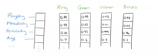
　　Word2Vec 是 Google 于 2013 年开源推出的一款将词表征为实数值向量的高效工具，采用的模型有CBOW（Continuous Bag-Of-Words，连续的词袋模型）和Skip-gram两种。Word2Vec通过训练，可以把对文本内容的处理简化为K维向量空间中的向量运算，而向量空间上的相似度可以用来表示文本语义上的相似度。因此，Word2Vec输出的词向量可以被用来做很多NLP相关的工作，比如聚类、找同义词、词性分析等等。经过训练，部分单词向量的加法组合运算能达到类似于下面公式的效果：

　　vector('Paris') - vector('France') + vector('Italy') ≈ vector('Rome')

　　此外，下图也简洁明了的展示的Word2Vec的词向量特征。

　　Word2Vec受欢迎的另一个原因是它的高效，具体思想可由Tomas Mikolov的两篇论文一探究竟。此文是我对Word2Vec学习的笔记。

二、分布式词表示（Distributed Representation）

　   自然语言处理的相关任务中，要想将自然语言处理交给机器学习中的算法处理，首先应该将语言数学化。在计算机运算中，向量可以说是人对机器输入的主要方式。而词向量，顾名思义，就是把一个词表示成一个向量，主要分为两种表示方法：One-Hot Representation 和 Distributed Representation。

　　我们知道，最简单的一种词表示方式是One-Hot表示，它的优点是很容易表示出不同的词，但是缺点也是巨大的：一、所有词向量正交，即无法刻画词与词之间的相似性。二、当有非常大的数据量时，向量的维度会因此扩大而造成维度灾难。如下所示，如果用One-Hot方式来表示自然界生物，自然界的动物种类数以百万记，因为数据量庞大，基本不可能用这种方式来表示动物类别，并且也无法表示诸如河虾、鲤鱼都生活在水里的这一相似性。

　　　　鳄鱼    [1,0,0,0,0,0,……,0,0,0,0,0,0,0]

　　　　天鹅    [0,1,0,0,0,0,……,0,0,0,0,0,0,0]

　　　　鲤鱼    [0,0,0,0,1,0,……,0,0,0,0,0,0,0]

　　　　河虾    [0,0,0,0,0,0,……,1,0,0,0,0,0,0]

　　　　…

 　　      老虎    [0,0,0,0,0,0,……,0,0,0,0,0,0,1]

 　　分布式词表示使用低维、稠密、连续的向量来表示词。最早由Hinton 于 1986年提出，可以克服 one-hot representation 的缺点。它们通过“有指导”的方法直接学习词向量，也称为词嵌入（Word Embedding）。它的发展历程由最初的LSA、LDA、NNLM发展到后来的诸如RNNLM、Word2Vec、GloVe，以及现在最新的ELMo和BERT，应当注意每个词在不同的语料库和不同的训练方法下，得到的词向量是不一样的。

由于是用向量表示，通过训练算法得到的词向量的向量一般在空间上是有意义的。分布式词可以用较低维度的矩阵去表示一个词，并且“赋予”矩阵各行列有各自的意义，词与词之间的相似度也可以通过矩阵运算来求得。也就是说，所有的词经过训练后形成以个词向量空间，而每一向量对应空间中一点，在这个空间上词向量之间的距离度量也可以表示对应的两个词之间的“距离”。那么这个距离就是两词之间的语法、语义的相似性代数表示。

　　词向量在机器翻译领域的一个应用，是有google的Mikolov团队开发一种词典和术语表示的自动生成技术，该技术也是利用词向量空间，能把一种语言转变成另一种语言，利用了不同语言在向量空间上的坐标“相对位置”类似，实验中对英语和西班牙语之间的翻译准确率高达90%。

　　介绍算法原理的时候举出一下例子：通过训练得到英语、西班牙语的对应的词向量空间E和S。 从英语中取出五个词 one 、two、three、four、five，设其在E中对应的词向量分别为v1、v2、v3、v4、v5，为方便作图，利用主成分分析(PCA)降维，得到相应的二维向量u1、u2、u3、u4、u5，在二维平面将这5个点描出来。类似地应用此方法，得到西语降维后的二维向量t1、t2、t3、t4、t5，如下图所示。

 

 

　　

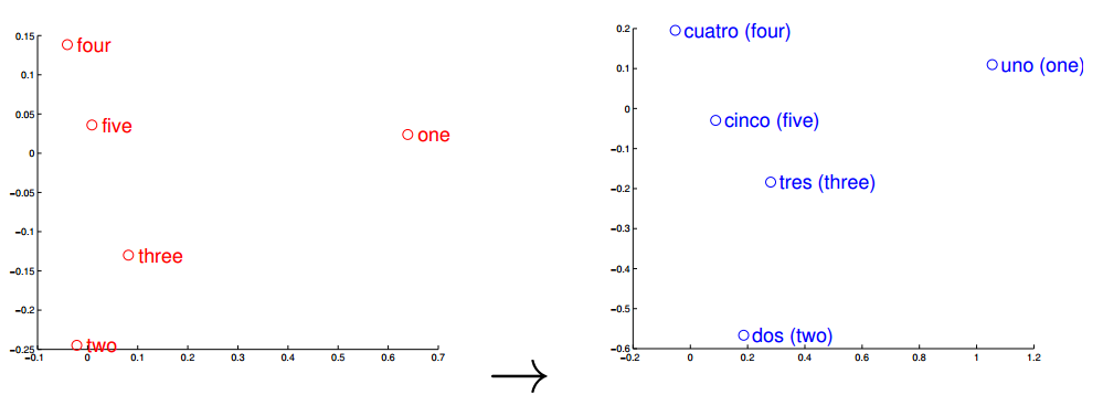
　　观察左右两图，可以发现：五个词在两个向量空间的相对位置差不多，说明了两种语言对应向量空间结构之间具有相似性，进一步说明词向量在刻画词与词相关性是合理的。

   

三、CBOW与skip-gram

　　语言模型形式化的描述就是给定一个T个词的字符串s，看他是自然语言的概率。举个例子：P（我，爱，学习，机器学习）= P（我）P（爱 | 我）P（学习 | 我，爱）P（机器学习 | 我，爱，学习）。这就是一种上下文相关的语言模型。但当碰到一个很长的语料，如果把一个词的出现要和前边所有出现过的单词联系起来，是非常复杂并且难以计算的。19世纪到20世纪初，俄罗斯数学家马尔科夫(Andrey Markov) 提出：假设任意一个词 wt 出现的概率只同他前面的词 wt-1 有关，问题就变得简单了。这种假设在数学上称为马尔科夫假设。

　　CBOW全称Continuous Bag-of-Words Model，Skip-Gram全称Continuous skip-gram Model。两者是Word2Vec里重要的两种模型，CBOW模型的训练输入是某一个特征词的上下文相关的词对应的词向量，而输出就是这特定的一个词的词向量。Skip-Gram模型和CBOW的思路是反着来的，即输入是特定的一个词的词向量，而输出是特定词对应的上下文词向量。这两种模型都包含三层，输入层、投影层、输出层：

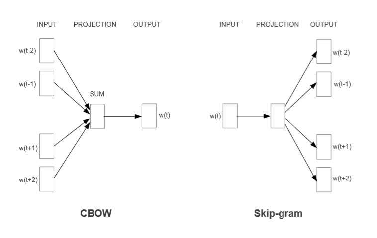
由上图可见，CBOW是在已知当前词 wt 的上下文 wt-2,wt-1,wt+1,wt+2 的前提下预测当前词wt；而Skip-gram则是已知当前词 wt 的前提下 ，去预测 wt-2,wt-1,wt+1,wt+2 。

 

四、Hierarchical Softmax框架与Negative Sampling框架

　　这两者并不是Word2Vec的精髓，只是Word2Vec的训练技巧。Hierarchical Softmax本质是把 N 分类问题变成 log(N) 次二分类； Negative Sampling 本质是预测总体类别的一个子集。

　　Hierarchical Softmax 和 Negative Sampling是Word2Vec设计的两种实现框架。Hierachical Softmax的基本思想是：它把训练语料中的词当成叶子节点，其在语料中出现的次数当做权值，通对于词典Dictionary中的任意词 w，Huffman 树中必存在一条从根节点到词 w 对应结点的路径，由此每个词对应一个Huffman编码。而 Negative Sampling 不再使用复杂的 Huffman树，而是采用随机负采样，可以减少训练时间和大幅度提高性能。

　　何为负采样算法呢？训练一个神经网络，样本只要有所改变（添加、修改、删除）就需要稍微调整所有的神经网络权重，这样才能确保训练结果的准确性。如果有一个巨大数据集，一个样本的改变都会改变神经网络的权重，代价是高昂的。而负采样的好处是，每一个训练样本仅仅改变一小部分的权重而不是所有的权重，解决了这个问题。比如，当我要进行对 ”ready“ 这个单词进行训练时，使用负采样，随机选择较少数目（小样本一般为5~20个，大样本为2~5个）的 ”负“ 样本进行权重更新，并且仍然为我们的 ”正“ 单词更新其对应的权重。词典 Dictionary 中的词在语料Corpus中出现的次数不同，那么对于高频词而言，被选为负样本的概率就应该比较大，而对于低频词，被选中的概率就应该小。

　　如果我们的输出层大约有 300 x 10,000 维度的权重矩阵，对 ”quick“ 一次进行权重更新，加上额外5个 负样本的权重更新，一共是6个输出神经元，和1800个权重值。这些值，仅仅只占输出层 3,000,000 神经元中的 0.06%。

五、代码实现

　　此代码已上传github，点击此处查看。网上有很多关于Word2Vec的实现，本文最初参考此代码以及一些现成代码，在后边的参考文章中列举。

import collections
import math
import os
import random
import zipfile
import numpy as np
import urllib
import tensorflow as tf
import matplotlib.pyplot as plt
from sklearn.manifold import TSNE

# Step 1 : 准备数据文档

url = 'http://mattmahoney.net/dc/'

def download_check(filename, expected_bytes):
    """下载数据集，如果存在就确认跳过."""
    if not os.path.exists(filename):
        print('正在下载所需数据包 …')
        filename, _ = urllib.request.urlretrieve(url + filename, filename)
    statinfo = os.stat(filename)
    if statinfo.st_size == expected_bytes:
        print('确认为目标文件 ', filename)
    else:
        print(statinfo.st_size)
        raise Exception(
            '文件大小不对应 ' + filename + '请前往 http://mattmahoney.net/dc/text8.zip 获取数据集')
    return filename

filename = download_check('text8.zip', 31344016)

# Step 2 ： 解压文件

def read_data(filename):
    """读取zip的第一个文件并且分割单词为字符串数组"""
    with zipfile.ZipFile(filename) as f:
        data = tf.compat.as_str(f.read(f.namelist()[0])).split()
    return data

words = read_data(filename)
print('数据长度', len(words))

vocabulary_size = 50000

# Step 3 ： 准备数据集

def build_dataset(words):
    """在字典第一个位置插入一项“UNK"代表不能识别的单词，也就是未出现在字典的单词统一用UNK表示"""
#  [['UNK', -1], ['i', 500], ['the', 498], ['man', 312], ...]
    count = [['UNK', -1]]
#  dictionary {'UNK':0, 'i':1, 'the': 2, 'man':3, ...} 收集所有单词词频
    count.extend(collections.Counter(words).most_common(vocabulary_size - 1))
#  python中K/V的一种数据结构"字典
    dictionary = dict()
    for word, _ in count:
        dictionary[word] = len(dictionary)
    data = list()
    unk_count = 0
    for word in words:
        if word in dictionary:
            index = dictionary[word]
        else:
            index = 0 # dictionary['UNK']
            unk_count += 1
        data.append(index)
    count[0][1] = unk_count
    reverse_dictionary = dict(zip(dictionary.values(), dictionary.keys()))
    return data, count, dictionary, reverse_dictionary

data, count, dictionary, reverse_dictionary = build_dataset(words)

del words
print('词频最高的词', count[:5])
print('数据样例', data[:10], [reverse_dictionary[i] for i in data[:10]])

data_index = 0

# Step 4 : skip-gram

def generate_batch(batch_size, num_skips, skip_window):
    global data_index #global关键字 使data_index 可在其他函数中修改其值
    assert batch_size % num_skips == 0 #assert断言用于判断后者是否为true，如果返回值为假，处罚异常
    assert num_skips <= 2 * skip_window
    batch = np.ndarray(shape=(batch_size), dtype=np.int32) #ndarray对象用于存放多维数组
    labels = np.ndarray(shape=(batch_size, 1), dtype=np.int32)
    span = 2 * skip_window + 1 # [ skip_window target skip_window]
    # 初始化最大长度为span的双端队列，超过最大长度后再添加数据，会从另一端删除容不下的数据
    # buffer: 1, 21, 124, 438, 11
    buffer = collections.deque(maxlen=span) #创建一个队列,模拟滑动窗口
    for _ in range(span):
        buffer.append(data[data_index])
        data_index = (data_index + 1) % len(data)
    for i in range(batch_size // num_skips): # // 是整数除
        # target : 2
        target = skip_window # target label at the center of the buffer
        # target_to_avoid : [2]
        targets_to_avoid = [ skip_window ] # 需要忽略的词在当前的span位置
        # 更新源单词为当前5个单词的中间单词
        source_word = buffer[skip_window]
        # 随机选择的5个span单词中除了源单词之外的4个单词中的两个
        for j in range(num_skips):
            while target in targets_to_avoid:
                target = random.randint(0, span - 1)
            targets_to_avoid.append(target) # 已经经过的target放入targets_to_avoid
            #batch中添加源单词
            batch[i * num_skips + j] = source_word
            #labels添加目标单词，单词来自随机选择的5个span单词中除了源单词之外的4个单词中的两个
            labels[i * num_skips + j, 0] = buffer[target]
        # 往双端队列中添加下一个单词，双端队列会自动将容不下的数据从另一端删除
        buffer.append(data[data_index])
        data_index = (data_index + 1) % len(data)
    return batch, labels

# Step 5 : 构建一个包含隐藏层的神经网络，隐藏层包含300节点，与我们要构造的WordEmbedding维度一致

batch, labels  = generate_batch(batch_size=8, num_skips=2, skip_window=1)
# 打印数据样例中的skip-gram样本
for i in range(8):
    print('(',batch[i], reverse_dictionary[batch[i]],
    ',', labels[i, 0], reverse_dictionary[labels[i, 0]],')')
"""
( 3081 originated , 12 as )
( 3081 originated , 5234 anarchism )
( 12 as , 6 a )
( 12 as , 3081 originated )
( 6 a , 12 as )
( 6 a , 195 term )
( 195 term , 6 a )
( 195 term , 2 of )
"""
batch_size = 128
embedding_size = 128 # Demension of the embedding vector
skip_window = 1      # How many words to consider left and right
num_skips = 2        # How many times to reuse an input to generate a label

valid_size = 16      # Random set of words to evaluate similarity on
valid_window = 100   # Only pick dev samples in the head of the distribution
valid_examples = np.random.choice(valid_window, valid_size, replace=False)
num_sampled = 64     # Number of negative examples to sample

graph = tf.Graph()
with graph.as_default():
    # 定义输入输出
    train_inputs = tf.placeholder(tf.int32, shape=[batch_size])
    train_labels = tf.placeholder(tf.int32, shape=[batch_size, 1])
    valid_dataset = tf.constant(valid_examples, dtype=tf.int32)

    # 当缺少GPU时，用CPU来进行训练和操作变量
    with tf.device('/cpu:0'):
        # 初始化embedding矩阵，后边经过多次训练后我们得到的结果就放在此embedding矩阵;
        # tf.Variable是图变量，tf.radom_uniform产生一个在[-1,1]间均匀分布的size为[vocabulary_size, embedding_size]的矩阵
        embeddings = tf.Variable(
            tf.random_uniform([vocabulary_size, embedding_size], -1.0, 1.0))
        # 将输入序列转换成embedding表示, [batch_size, embedding_size]
        # tf.nn.embedding_lookup的作用就是找到要寻找的embedding data中的对应的行下的vector
        emded = tf.nn.embedding_lookup(embeddings, train_inputs)

        # 初始化权重，此处使用负例采样NCE loss损失函数
        # tf.truncated_normal(shape, mean, stddev) :shape表示生成张量的维度，mean是均值，stddev是标准差。这个函数产生正太分布，
        # 均值和标准差自己设定。这是一个截断的产生正太分布的函数，就是说产生正太分布的值如果与均值的差值大于两倍的标准差，那就重新生成。
        nce_weights = tf.Variable(
            tf.truncated_normal([vocabulary_size, embedding_size],
                                stddev=1.0 / math.sqrt(embedding_size)))
        nce_biases = tf.Variable(tf.zeros([vocabulary_size]))
    # Compute the average NCE loss for the batch
    # tf.nce_loss automatically draws a new sample of the negative labels each
    # time we evalute the loss
    loss =  tf.reduce_mean(
        tf.nn.nce_loss(weights = nce_weights,
                       biases = nce_biases,
                       labels = train_labels,
                       inputs = emded,
                       num_sampled = num_sampled,
                       num_classes = vocabulary_size ))
        # 使用1.0的速率来构造SGD优化器
    optimizer = tf.train.GradientDescentOptimizer(1.0).minimize(loss)
        # 计算 minibatch 和 all embeddings的余弦相似度
        # tf.reduce_sum() 按照行的维度求和
    norm = tf.sqrt(tf.reduce_sum(tf.square(embeddings), 1, keep_dims=True))
    normalized_embeddings = embeddings / norm
    valid_embeddings = tf.nn.embedding_lookup(normalized_embeddings, valid_dataset)
        # tf.matmul 矩阵相乘
    similarity = tf.matmul(valid_embeddings, normalized_embeddings, transpose_b=True)
        # 添加变量初始化程序
    init = tf.global_variables_initializer()

# Step 6 : 开始训练
# 训练次数
num_steps = 100001
    # tf.Session 用于运行TensorFlow操作的类
with tf.Session(graph=graph) as session:
    # 我们必须在使用之前初始化所有变量
    init.run()
    print("Initialized")
    average_loss = 0
    for step in range(num_steps):
        batch_inputs, batch_labels = generate_batch(
            batch_size, num_skips, skip_window)
        feed_dict = {train_inputs : batch_inputs, train_labels : batch_labels}
        # We perform one update step by evaluating the optimizer op( including it
        # in the list of returned values for session.run())
        _, loss_val = session.run([optimizer, loss], feed_dict=feed_dict)
        average_loss += loss_val
        if step % 2000 == 0:
            if step > 0:
                average_loss /= 2000
            #The average loss is an estimate of the loss over the last 2000 batches.
            print("Average loss at step", step, ": ", average_loss)
            average_loss = 0
        # Note that this is expensive ( ~20% slowdown if computed every 500 steps)
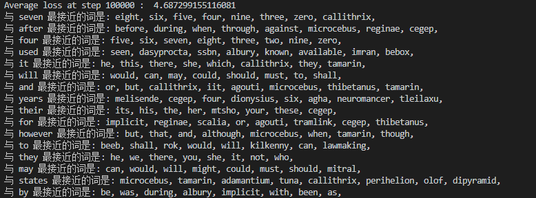
        if step % 10000 == 0:
            sim = similarity.eval()
            for i in range(valid_size):
                valid_word = reverse_dictionary[valid_examples[i]]
                top_k = 8 # number of nearest neighbors
                nearest = (-sim[i, : ]).argsort()[1:top_k+1]
                log_str = "与 %s 最接近的词是:" % valid_word
                for k in range(top_k):
                    close_word = reverse_dictionary[nearest[k]]
                    log_str = "%s %s," % (log_str, close_word)
                print(log_str)
    final_embeddings = normalized_embeddings.eval()

# Step 7 ： 绘制结果
def plot_with_labels(low_dim_embs, labels, filename='TSNE_result.png'):
    assert low_dim_embs.shape[0] >= len(labels), "More labels than embeddings"
    plt.figure(figsize=(18, 18)) # in inches
    for i, label in enumerate(labels):
        x, y = low_dim_embs[i,:]
        plt.scatter(x, y)
        plt.annotate(label,
                    xy=(x, y),
                    xytext=(5, 2),
                    textcoords='offset points',
                    ha='right',
                    va='bottom')
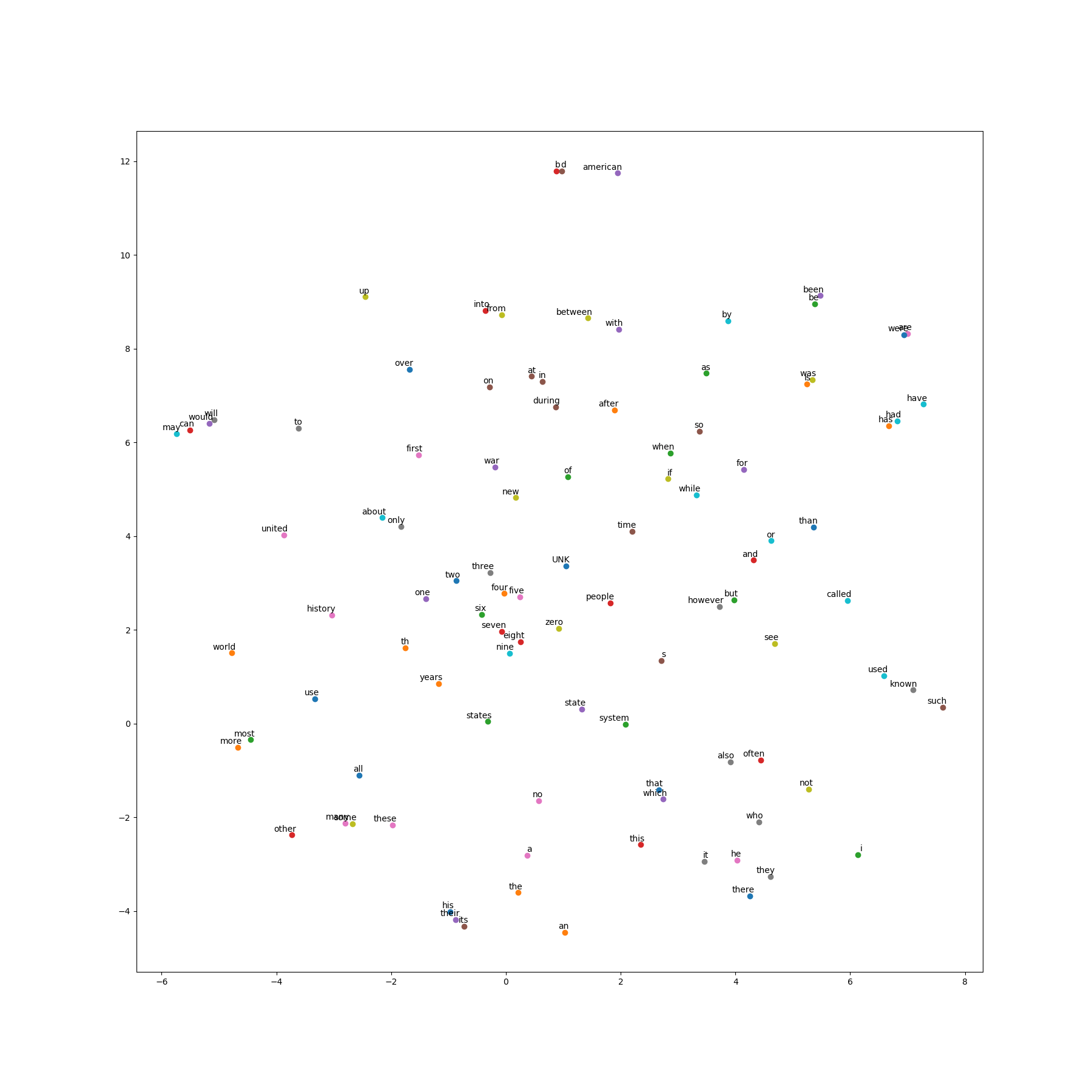
    plt.savefig(filename)

# 使用T-SNE算法将128维降低到2维
tsne = TSNE(perplexity= 30, n_components = 2, init = 'pca', n_iter = 5000, random_state = 1)
# 绘制点的个数
plot_only = 100
low_dim_embs = tsne.fit_transform(final_embeddings[: plot_only, :])
labels = [reverse_dictionary[i] for i in range(plot_only)]
plot_with_labels(low_dim_embs, labels)
plt.show()

 

六、训练结果

参考资料：

1、https://www.jianshu.com/p/471d9bfbd72f

2、https://www.jianshu.com/p/0bb00eed9c63

3、https://blog.csdn.net/itplus/article/details/37998797

4、https://blog.csdn.net/qq_28444159/article/details/77514563