Approximate Nearest Neighbors.接近最近邻搜索

（一）：次优最近邻：http://en.wikipedia.org/wiki/Nearest_neighbor_search

有少量修改；如有疑问，请看链接原文.....
1.Survey:
Nearest neighbor search (NNS), also known as proximity search,similarity search orclosest point search,
is anoptimization problem for finding closest (or most similar) points. Closeness is typically expressed in terms of a dissimilarity
function: The less similar are the objects the larger are the function values. Formally, the nearest-neighbor (NN) search problem is defined as follows: given a setS of points in a spaceM and a query pointq ∈ M, find the
closest point inS toq. Donald Knuth in vol. 3 of The Art of Computer Programming (1973) called it thepost-office problem,
referring to an application of assigning to a residence the nearest post office. A direct generalization of this problem is ak-NN search, where we need to find thek closest points.寻找高维近邻点的最优化问题；

Most commonly M is a metric space and dissimilarity is expressed as a distance metric, which is symmetric and satisfies the triangle inequality. Even more common, M is taken to be the d-dimensionalvector space where dissimilarity is measured using theEuclidean
distance, Manhattan distance or other distance metric. However, the dissimilarity function can be arbitrary. One example are asymmetricBregman divergences, for which the
triangle inequality does not hold.^[1]

距离矩阵的度量问题；

2.方法：(遇到的问题：维数灾难；)

Linear search(适合小范围的距离计算)

The simplest solution to the NNS problem is to compute the distance from the query point to every other point in the database, keeping track of the "best so far". This algorithm, sometimes referred
to as the naive approach, has a running time of O(Nd) where N is the cardinality of S and d is the dimensionality of M. There are no search data structures to maintain, so linear search has no space complexity beyond the storage of the database. Naive search can, on average, outperform space partitioning
approaches on higher dimensional spaces.^[2]

Space partitioning（决策树？）

Since the 1970s, branch and bound methodology has been applied to the problem. In the case of Euclidean space this approach is known asspatial
index or spatial access methods. Several space-partitioning methods have been developed for solving the NNS problem. Perhaps the simplest is thek-d tree, which iteratively bisects the search space
into two regions containing half of the points of the parent region. Queries are performed via traversal of the tree from the root to a leaf by evaluating the query point at each split. Depending on the distance specified in the query, neighboring branches
that might contain hits may also need to be evaluated. For constant dimension query time, average complexity isO(log N)^[3]
in the case of randomly distributed points, worst case complexity analyses have been performed.^[4]
Alternatively theR-tree data structure was designed to support nearest neighbor search in dynamic context, as it has efficient algorithms for insertions and deletions.

In case of general metric space branch and bound approach is known under the name ofmetric
trees. Particular examples include vp-tree and BK-tree.

Using a set of points taken from a 3-dimensional space and put into aBSP
tree, and given a query point taken from the same space, a possible solution to the problem of finding the nearest point-cloud point to the query point is given in the following description of an algorithm. (Strictly speaking, no such point may exist,
because it may not be unique. But in practice, usually we only care about finding any one of the subset of all point-cloud points that exist at the shortest distance to a given query point.) The idea is, for each branching of the tree, guess that the closest
point in the cloud resides in the half-space containing the query point. This may not be the case, but it is a good heuristic. After having recursively gone through all the trouble of solving the problem for the guessed half-space, now compare the distance
returned by this result with the shortest distance from the query point to the partitioning plane. This latter distance is that between the query point and the closest possible point that could exist in the half-space not searched. If this distance is greater
than that returned in the earlier result, then clearly there is no need to search the other half-space. If there is such a need, then you must go through the trouble of solving the problem for the other half space, and then compare its result to the former
result, and then return the proper result. The performance of this algorithm is nearer to logarithmic time than linear time when the query point is near the cloud, because as the distance between the query point and the closest point-cloud point nears zero,
the algorithm needs only perform a look-up using the query point as a key to get the correct result.

空间划分是一个构建空间树的过程，其构建过程比较复杂，涉及到大量的计算；

Locality sensitive hashing（hash过程，可以近似O(1)的时间查询表）

Locality sensitive hashing (LSH) is a technique
for grouping points in space into 'buckets' based on some distance metric operating on the points. Points that are close to each other under the chosen metric are mapped to the same bucket with high probability.^[5]

Nearest neighbor search in spaces with small intrinsicdimension

The cover tree has a theoretical bound that is based on the dataset's doubling constant. The bound on search time is O(c¹² log n) wherec is theexpansion
constant of the dataset.

Vector approximation files

In high dimensional spaces, tree indexing structures become useless because an increasing percentage of the nodes need to be examined anyway. To speed up linear search, a compressed version of the
feature vectors stored in RAM is used to prefilter the datasets in a first run. The final candidates are determined in a second stage using the uncompressed data from the disk for distance calculation.^[6]

Compression/clustering based search

The VA-file approach is a special case of a compression based search, where each feature component is compressed uniformly and independently. The optimal compression technique in multidimensional
spaces is Vector Quantization (VQ), implemented through clustering. The database is clustered and the most "promising" clusters are retrieved. Huge gains over VA-File, tree-based indexes and sequential scan have been observed.^[7][8]
Also note the parallels between clustering and LSH.

3.次优最近邻

Algorithms that support the approximate nearest neighbor search includelocality-sensitive
hashing,best bin first andbalanced
box-decomposition tree based search.^[9]

(1):ε-approximate nearest neighbor search is a special case of thenearest neighbor search problem. The solution
to the ε-approximate nearest neighbor search is a point or multiple points within distance (1+ε) R from a query point, where R is the distance between the query point and its true nearest neighbor.

Reasons to approximate nearest neighbor search include the space and time costs of exact solutions in high dimensional spaces (seecurse
of dimensionality) and that in some domains, finding an approximate nearest neighbor is an acceptable solution.

Approaches for solving
ε-approximate nearest neighbor search includekd-trees,Locality
Sensitive Hashing andbrute force search.

(2):

Best bin first is a
search algorithm that is designed to efficiently find an approximate solution to the
nearest neighbor search problem in very-high-dimensional spaces. The algorithm is based on a variant of thekd-tree
search algorithm which makes indexing higher dimensional spaces possible. Best bin first is an approximate algorithm which returns the nearest neighbor for a large fraction of queries and a very close neighbor otherwise.^[1]

Differences from kd tree:

• Backtracking is according to a priority queue based on closeness.
• Search a fixed number of nearest candidates and stop.
• A speedup of two orders of magnitude is typical.                                        主要是对于超大型数据库进行相似性查询；

References:Beis, J.; Lowe, D. G. (1997). "Shape indexing
using approximate nearest-neighbour search in high-dimensional spaces". Conference on Computer Vision and Pattern Recognition. Puerto Rico. pp. 1000–1006.CiteSeerX:10.1.1.23.9493.

(3):LSH:http://en.wikipedia.org/wiki/Locality_sensitive_hashing
Locality-sensitive hashing (LSH) is a method of performing probabilisticdimension reduction
of high-dimensional data. The basic idea is tohash the input items so that similar items are mapped to the same buckets with
high probability (the number of buckets being much smaller than the universe of possible input items). This is different from the conventional hash functions, such as those used incryptography,
as in the LSH case the goal is to maximize probability of "collision" of similar items rather than avoid collisions.^[1]
Note how locality-sensitive hashing, in many ways, mirrors data clustering andNearest neighbor search.



（二）：局部敏感hash：

（三）：minihash：原文链接：http://my.oschina.net/pathenon/blog/65210
转自wiki：http://en.wikipedia.org/wiki/Locality_sensitive_hashing

    传统的hash算法只负责将原始内容尽量均匀随机地映射为一个签名值，原理上相当于伪随机数产生算法。传统hash算法产生的两个签名，如果相等，说明原始内容在一定概率下是相等的；如果不相等，除了说明原始内容不相等外，不再提供任何信息，因为即使原始内容只相差一个字节，所产生的签名也很可能差别极大。从这个意义上来说，要设计一个hash算法，对相似的内容产生的签名也相近，是更为艰难的任务，因为它的签名值除了提供原始内容是否相等的信息外，还能额外提供不相等的原始内容的差异程度的信息。

    MinHash^[1最小哈希方法可看作是局部性敏感哈希的一个实例。局部性敏感哈希是使用哈希将大集合的数据对象映射到更小的哈希值的技术集合，通过这样的方法当两个对象距离相近时，它们的哈希值也可以相同。在最小哈希方法实例中，一个集合的签名可看作是它的哈希值。其它局部性敏感哈希技术还有针对集合间的海明距离，以及向量间的余弦距离等。另外，局部性敏感哈希还在最近邻搜索算法有着重要的应用。^[9]

1.概述introduction：

    跟SimHash一样，MinHash也是LSH的一种，可以用来快速估算两个集合的相似度。MinHash由Andrei
Broder提出，最初用于在搜索引擎中检测重复网页。它也可以应用于大规模聚类问题。

2.Jaccard index：雅可比相似度与最小哈希值

      在介绍MinHash之前，我们先介绍下Jaccard index。

Jaccard index是用来计算相似性，也就是距离的一种度量标准。假如有集合A、B，那么，

      也就是说，集合A,B的Jaccard系数等于A,B中共同拥有的元素数与A,B总共拥有的元素数的比例。很显然，Jaccard系数值区间为[0,1]。

假定h是一个将A和B中的元素映射到一些不相交整数的哈希函数，而且针对给定的S，定义h_min(S)为S集合中具有最小h(x)函数值的元素x。这样，只有当最小哈希值的并集A
∪ B依赖于交集A ∩B时，有h_min(A) =h_min(B)。 因此，

Pr[h_min(A) =h_min(B)] =J(A,B).

另一方面来说，如果r是一个当h_min(A) =h_min(B)时值为1，其它情况下值为0的随机变量，那么r可认为是J(A,B)的无偏估计。尽管此时方差过高，单独使用时没什么用处。最小哈希方法的思想是通过平均用同一方式构造的许多随机变量，从而减少方差。

3.MinHash：多哈希函数，单一哈希函数：

    先定义几个符号术语：

    h(x):  把x映射成一个整数的哈希函数。   

    h_min(S)：集合S中的元素经过h(x)哈希后，具有最小哈希值的元素。

那么对集合A、B，h_min(A) = h_min(B)成立的条件是A ∪ B 中具有最小哈希值的元素也在 ∩ B中。这里有一个假设，h(x)是一个良好的哈希函数，它具有很好的均匀性，能够把不同元素映射成不同的整数。

所以有，Pr[h_min(A)
= h_min(B)] = J(A,B)，即集合A和B的相似度为集合A、B经过hash后最小哈希值相等的概率。

   有了上面的结论，我们便可以根据MinHash来计算两个集合的相似度了。一般有两种方法：

第一种：使用多个hash函数

        为了计算集合A、B具有最小哈希值的概率，我们可以选择一定数量的hash函数，比如K个。然后用这K个hash函数分别对集合A、B求哈希值，对

每个集合都得到K个最小值。比如Min(A)k={a1,a2,...,ak}，Min(B)k={b1,b2,...,bk}。

        那么，集合A、B的相似度为|Min(A)k ∩ Min(B)k|
/ |Min(A)k  ∪  Min(B)k|，及Min(A)k和Min(B)k中相同元素个数与总的元素个数的比例。

第二种：使用单个hash函数

    第一种方法有一个很明显的缺陷，那就是计算复杂度高。使用单个hash函数是怎么解决这个问题的呢？请看：

   前面我们定义过 h_min(S)为集合S中具有最小哈希值的一个元素，那么我们也可以定义h_mink(S)为集合S中具有最小哈希值的K个元素。这样一来，

我们就只需要对每个集合求一次哈希，然后取最小的K个元素。计算两个集合A、B的相似度，就是集合A中最小的K个元素与集合B中最小的K个元素

的交集个数与并集个数的比例。

        

     看完上面的，你应该大概清楚MinHash是怎么回事了。但是，MinHash的好处到底在哪里呢？计算两篇文档的相似度，就直接统计相同的词数和总的

次数，然后就Jaccard index不就可以了吗？对，如果仅仅对两篇文档计算相似度而言，MinHash没有什么优势，反而把问题复杂化了。但是如果有海量的文档需要求相似度，比如在推荐系统

中计算物品的相似度，如果两两计算相似度，计算量过于庞大。下面我们看看MinHash是怎么解决问题的。

     比如元素集合{a,b,c,d,e},其中s1={a,d},s2={c},s3={b,d,e},s4={a,c,d} 那么这四个集合的矩阵表示为： 

       如果要对某一个集合做MinHash，则可以从上面矩阵的任意一个行排列中选取一个，然后MinHash值是排列中第一个1的行号。

    例如，对上述矩阵，我们选取排列
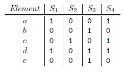
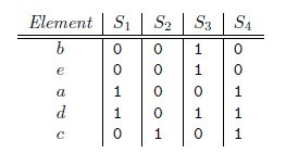
beadc，那么对应的矩阵为

        

        那么，
h(S1) = a，同样可以得到h(S2) = c, h(S3) = b, h(S4) = a。

        如果只对其中一个行排列做MinHash，不用说，计算相似度当然是不可靠的。因此，我们要选择多个行排列来计算MinHash，最后根据Jaccard index公式来计算相似度。但是求排列本身的复杂度比较高，特别是针对很大的矩阵来说。因此，我们可以设计一个随机哈希函数去模拟排列，能够把行号0~n随机映射到0~n上。比如H(0)=100,H(1)=3...。当然，冲突是不可避免的，冲突后可以二次散列。并且如果选取的随机哈希函数够均匀，并且当n较大时，冲突发生的概率还是比较低的。

        说到这里，只是讨论了用MinHash对海量文档求相似度的具体过程，但是它到底是怎么减少复杂度的呢？

        比如有n个文档，每个文档的维度为m，我们可以选取其中k个排列求MinHash，由于每个对每个排列而言，MinHash把一篇文档映射成一个整数，所以对k个排列计算MinHash就得到k个整数。那么所求的MinHash矩阵为n*k维，而原矩阵为n*m维。n>>m时，计算量就降了下来。

    

4.参考文献

     (1):http://en.wikipedia.org/wiki/MinHash

              (2)  :http://fuliang.iteye.com/blog/1025638

              (3)：^Chum,
Ond?ej; Philbin, James; Isard, Michael; Zisserman, Andrew, Scalable near identical image and shot detection, Proceedings of the 6th ACM International Conference on Image and Cideo Retrieval (CIVR'07). 2007,doi:10.1145/1282280.1282359;Chum,
Ond?ej; Philbin, James; Zisserman, Andrew,Near duplicate image detection: min-hash and tf-idf weighting, Proceedings of the British
Machine Vision Conference,