TensorFlow技术解析与实战学习笔记（13）------Mnist识别和卷积神经网络AlexNet

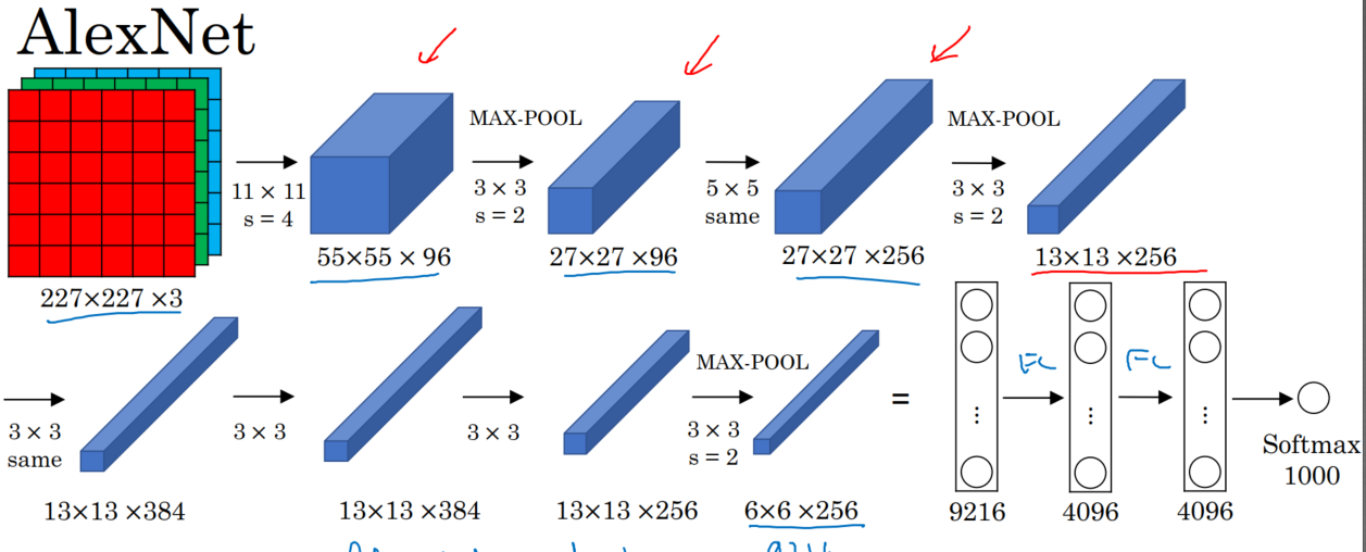
一、AlexNet：共8层：5个卷积层（卷积+池化）、3个全连接层，输出到softmax层，产生分类。

论文中lrn层推荐的参数：depth_radius = 4，bias = 1.0 , alpha = 0.001 / 9.0 , beta = 0.75

lrn现在仅在AlexNet中使用，主要是别的卷积神经网络模型效果不明显。而LRN在AlexNet中会让前向和后向速度下降，（下降1/3）。

【训练时耗时是预测的3倍】

代码：

#加载数据
import tensorflow as tf
from tensorflow.examples.tutorials.mnist import input_data
mnist = input_data.read_data_sets("MNIST_data/",one_hot = True)
 
#定义卷积操作
def conv2d(name , input_x , w , b , stride = 1,padding = 'SAME'):
    conv = tf.nn.conv2d(input_x,w,strides = [1,stride,stride,1],padding = padding , name = name)
    return tf.nn.relu(tf.nn.bias_add(conv,b))
def max_pool(name , input_x , k=2):
    return tf.nn.max_pool(input_x,ksize = [1,k,k,1],strides = [1,k,k,1],padding = 'SAME' , name = name)
def norm(name , input_x , lsize = 4):
    return tf.nn.lrn(input_x , lsize , bias = 1.0 , alpha = 0.001 / 9.0 , beta = 0.75 , name = name)
 
def buildGraph(x,learning_rate,weight,bias,dropout):
 
#############前向传播##################
    #定义网络
    x = tf.reshape(x , [-1,28,28,1])
    #第一层卷积
    with tf.variable_scope('layer1'):
        conv1 = conv2d('conv1',x,weight['wc1'],bias['bc1'])
        pool1 = max_pool('pool1',conv1)
        norm1 = norm('norm1',pool1)
    with tf.variable_scope('layer2'):
        conv2 = conv2d('conv2',norm1,weight['wc2'],bias['bc2'])
        pool2 = max_pool('pool2',conv2)
        norm2 = norm('norm2',pool2)
    with tf.variable_scope('layer3'):
        conv3 = conv2d('conv3',norm2,weight['wc3'],bias['bc3'])
        pool3 = max_pool('pool3',conv3)
        norm3 = norm('norm3',pool3)
    with tf.variable_scope('layer4'):
        conv4 = conv2d('conv4',norm3,weight['wc4'],bias['bc4'])
    with tf.variable_scope('layer5'):
        conv5 = conv2d('conv5',conv4,weight['wc5'],bias['bc5'])
        pool5 = max_pool('pool5',conv5)
        norm5 = norm('norm5',pool5)
    with tf.variable_scope('func1'):
        norm5 = tf.reshape(norm5,[-1,4*4*256])
        fc1 = tf.add(tf.matmul(norm5,weight['wf1']) , bias['bf1'])
        fc1 = tf.nn.relu(fc1)
        #dropout
        fc1 = tf.nn.dropout(fc1,dropout)
    with tf.variable_scope('func2'):
        fc2 = tf.reshape(fc1,[-1,weight['wf1'].get_shape().as_list()[0]])
        fc2 = tf.add(tf.matmul(fc1,weight['wf2']),bias['bf2'])
        fc2 = tf.nn.relu(fc2)
        #dropout
        fc2 = tf.nn.dropout(fc2,dropout)
    with tf.variable_scope('outlayer'):
        out = tf.add(tf.matmul(fc2,weight['w_out']),bias['b_out'])
    return out
 
def train(mnist):
        #定义网络的超参数
    learning_rate = 0.001
    training_step = 20000
    batch_size = 128
 
    #定义网络的参数
    n_input = 784
    n_output = 10
    dropout = 0.75
 
    #x、y的占位
    x = tf.placeholder(tf.float32,[None,784])
    y = tf.placeholder(tf.float32,[None,10])
    keep_prob = tf.placeholder(tf.float32)
 
    #权重和偏置的设置
    weight = {
        'wc1':tf.Variable(tf.truncated_normal([11,11,1,96],stddev = 0.1)),
        'wc2':tf.Variable(tf.truncated_normal([5,5,96,256],stddev = 0.1)),
        'wc3':tf.Variable(tf.truncated_normal([3,3,256,384],stddev = 0.1)),
        'wc4':tf.Variable(tf.truncated_normal([3,3,384,384],stddev = 0.1)),
        'wc5':tf.Variable(tf.truncated_normal([3,3,384,256],stddev = 0.1)),
        'wf1':tf.Variable(tf.truncated_normal([4*4*256,4096])),
        'wf2':tf.Variable(tf.truncated_normal([4096,4096])),
        'w_out':tf.Variable(tf.truncated_normal([4096,10]))
    }
    bias = {
        'bc1':tf.Variable(tf.constant(0.1,shape = [96])),
        'bc2':tf.Variable(tf.constant(0.1,shape =[256])),
        'bc3':tf.Variable(tf.constant(0.1,shape =[384])),
        'bc4':tf.Variable(tf.constant(0.1,shape =[384])),
        'bc5':tf.Variable(tf.constant(0.1,shape =[256])),
        'bf1':tf.Variable(tf.constant(0.1,shape =[4096])),
        'bf2':tf.Variable(tf.constant(0.1,shape =[4096])),
        'b_out':tf.Variable(tf.constant(0.1,shape =[10]))
    }
 
    out = buildGraph(x,learning_rate,weight,bias,keep_prob)
    ####################后向传播####################
    #定义损失函数
    loss = tf.reduce_mean(tf.nn.softmax_cross_entropy_with_logits(labels=y, logits=out))
    optimizer = tf.train.AdamOptimizer(learning_rate).minimize(loss)
 
    #评估函数
    correction = tf.equal(tf.argmax(out,1),tf.argmax(y,1))
    acc = tf.reduce_mean(tf.cast(correction,tf.float32))
#####################################开始训练##############################
 
    init = tf.global_variables_initializer()
 
    with tf.Session() as sess:
        sess.run(init)
        step = 1
        while step <= training_step:
            batch_x , batch_y = mnist.train.next_batch(batch_size)
            sess.run(out,feed_dict = {x:batch_x,y:batch_y,keep_prob:dropout})
            print(out.shape)
            sess.run(optimizer,feed_dict = {x:batch_x,y:batch_y,keep_prob:dropout})
            if step % 500 == 0:
                loss , acc = sess.run([loss,acc],feed_dict = {x:batch_x,y:batch_y,keep_prob:1})
                print(step,loss,acc)
            step += 1
    print(sess.run(acc,feed_dict = {x:mnist.test.images[:256],y:mnist.test.images[:256],keep_prob:1}))
 
if __name__=='__main__':
    train(mnist)