回归-LDA与QDA

作者：桂。

时间：2017-05-23  06:37:31

链接：http://www.cnblogs.com/xingshansi/p/6892317.html

---

前言

仍然是python库函数scikit-learn的学习笔记，内容Regression-1.2Linear and Quadratic Discriminant Analysis部分，主要包括：

　  1）线性分类判别(Linear discriminant analysis, LDA)

　　2）二次分类判别（Quadratic discriminant analysis, QDA）

　　3）Fisher判据

 一、线性分类判别

对于二分类问题，LDA针对的是：数据服从高斯分布，且均值不同，方差相同。

概率密度：

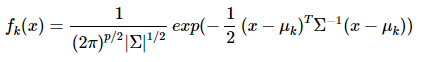
p是数据的维度。

分类判别函数：

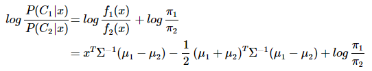
可以看出结果是关于x的一次函数：wx+w₀，线性分类判别的说法由此得来。

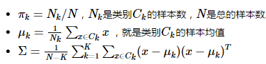
参数计算：

二、二次分类判别

对于二分类问题，QDA针对的是：数据服从高斯分布，且均值不同，方差不同。

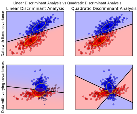
数据方差相同的时候，一次判别就可以，如左图所示;但如果方差差别较大，就是一个二次问题了，像右图那样。

从sklearn给的例子中，也容易观察到：

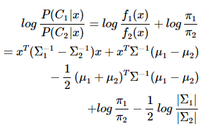
QDA对数据有更好的适用性，QDA判别公式：

三、Fisher判据

　　A-Fisher理论推导

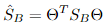
Fisher一个总原则是：投影之后的数据，最小化类内误差，同时最大化类间误差

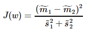
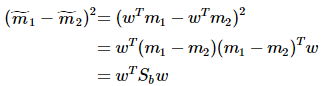
其中，，、分别对应投影后的类均值。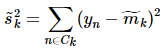对应投影后的类内方差。

重写类内总方差、类间距离：

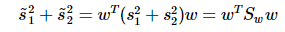
准则函数重写：

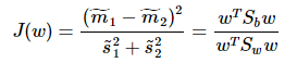
这就是泛化瑞利熵的形式了，容易求解：

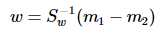
其中常借助SVD求解：Sw = U∑V^T，S_w^-1 = U∑^-1V^T,借助特征值分解也是可以的。

 　　B-LDA与Fisher

这里的LDA指代上面提到的利用概率求解的贝叶斯最优估计器。可以证明：

二分类任务中两类数据满足高斯分布且方差相同时，线性判别分析（指Fisher方法）产生贝叶斯最优分类器（指本文的LDA）。

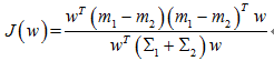
对于Fisher，求J的最大值：

贝叶斯最优，即距离分类中心距离除以两个类中心距离的比值最小：

二者倒数关系，一个最大化，一个最小化，所以是等价的。

补充一句：误差为高斯分布，与最小二乘也是等价的。

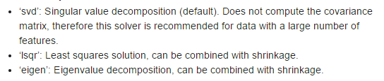
这样一来，求解就有了三个思路：奇异值分解SVD，最小二乘Lsqr，特征值分解eigen，这也是Sklearn的思路：

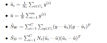
　　C-多分类LDA

定义类内散度矩阵：

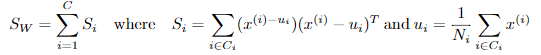
定义类间散度矩阵：

定义总散度矩阵：

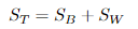
可见S_T 、S_B、 S_W三者任意取两个即可。

准则函数：

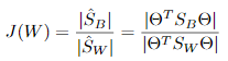
其中，。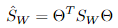

最优化求解：

将看作投影矩阵，其闭式解是的d'个最大非零广义特征值对应的特征向量组成的矩阵。d'通常远小于原数据属性数d，这就实现了监督的降维。

参数求解利用train data：

四、Sk-learn基本用法

　　LDA：

lda = LinearDiscriminantAnalysis(solver="svd", store_covariance=True)
y_pred = lda.fit(X, y).predict(X)

　　QDA：

qda = QuadraticDiscriminantAnalysis(store_covariances=True)
y_pred = qda.fit(X, y).predict(X)

　　LDA与QDA应用实例：

"""
====================================================================
Linear and Quadratic Discriminant Analysis with confidence ellipsoid
====================================================================
 
Plot the confidence ellipsoids of each class and decision boundary
"""
print(__doc__)
 
from scipy import linalg
import numpy as np
import matplotlib.pyplot as plt
import matplotlib as mpl
from matplotlib import colors
 
from sklearn.discriminant_analysis import LinearDiscriminantAnalysis
from sklearn.discriminant_analysis import QuadraticDiscriminantAnalysis
 
###############################################################################
# colormap
cmap = colors.LinearSegmentedColormap(
    'red_blue_classes',
    {'red': [(0, 1, 1), (1, 0.7, 0.7)],
     'green': [(0, 0.7, 0.7), (1, 0.7, 0.7)],
     'blue': [(0, 0.7, 0.7), (1, 1, 1)]})
plt.cm.register_cmap(cmap=cmap)
 
###############################################################################
# generate datasets
def dataset_fixed_cov():
    '''Generate 2 Gaussians samples with the same covariance matrix'''
    n, dim = 300, 2
    np.random.seed(0)
    C = np.array([[0., -0.23], [0.83, .23]])
    X = np.r_[np.dot(np.random.randn(n, dim), C),
              np.dot(np.random.randn(n, dim), C) + np.array([1, 1])]
    y = np.hstack((np.zeros(n), np.ones(n)))
    return X, y
 
def dataset_cov():
    '''Generate 2 Gaussians samples with different covariance matrices'''
    n, dim = 300, 2
    np.random.seed(0)
    C = np.array([[0., -1.], [2.5, .7]]) * 2.
    X = np.r_[np.dot(np.random.randn(n, dim), C),
              np.dot(np.random.randn(n, dim), C.T) + np.array([1, 4])]
    y = np.hstack((np.zeros(n), np.ones(n)))
    return X, y
 
###############################################################################
# plot functions
def plot_data(lda, X, y, y_pred, fig_index):
    splot = plt.subplot(2, 2, fig_index)
    if fig_index == 1:
        plt.title('Linear Discriminant Analysis')
        plt.ylabel('Data with fixed covariance')
    elif fig_index == 2:
        plt.title('Quadratic Discriminant Analysis')
    elif fig_index == 3:
        plt.ylabel('Data with varying covariances')
 
    tp = (y == y_pred)  # True Positive
    tp0, tp1 = tp[y == 0], tp[y == 1]
    X0, X1 = X[y == 0], X[y == 1]
    X0_tp, X0_fp = X0[tp0], X0[~tp0]
    X1_tp, X1_fp = X1[tp1], X1[~tp1]
 
    alpha = 0.5
 
    # class 0: dots
    plt.plot(X0_tp[:, 0], X0_tp[:, 1], 'o', alpha=alpha,
             color='red')
    plt.plot(X0_fp[:, 0], X0_fp[:, 1], '*', alpha=alpha,
             color='#990000')  # dark red
 
    # class 1: dots
    plt.plot(X1_tp[:, 0], X1_tp[:, 1], 'o', alpha=alpha,
             color='blue')
    plt.plot(X1_fp[:, 0], X1_fp[:, 1], '*', alpha=alpha,
             color='#000099')  # dark blue
 
    # class 0 and 1 : areas
    nx, ny = 200, 100
    x_min, x_max = plt.xlim()
    y_min, y_max = plt.ylim()
    xx, yy = np.meshgrid(np.linspace(x_min, x_max, nx),
                         np.linspace(y_min, y_max, ny))
    Z = lda.predict_proba(np.c_[xx.ravel(), yy.ravel()])
    Z = Z[:, 1].reshape(xx.shape)
    plt.pcolormesh(xx, yy, Z, cmap='red_blue_classes',
                   norm=colors.Normalize(0., 1.))
    plt.contour(xx, yy, Z, [0.5], linewidths=2., colors='k')
 
    # means
    plt.plot(lda.means_[0][0], lda.means_[0][1],
             'o', color='black', markersize=10)
    plt.plot(lda.means_[1][0], lda.means_[1][1],
             'o', color='black', markersize=10)
 
    return splot
 
def plot_ellipse(splot, mean, cov, color):
    v, w = linalg.eigh(cov)
    u = w[0] / linalg.norm(w[0])
    angle = np.arctan(u[1] / u[0])
    angle = 180 * angle / np.pi  # convert to degrees
    # filled Gaussian at 2 standard deviation
    ell = mpl.patches.Ellipse(mean, 2 * v[0] ** 0.5, 2 * v[1] ** 0.5,
                              180 + angle, facecolor=color, edgecolor='yellow',
                              linewidth=2, zorder=2)
    ell.set_clip_box(splot.bbox)
    ell.set_alpha(0.5)
    splot.add_artist(ell)
    splot.set_xticks(())
    splot.set_yticks(())
 
def plot_lda_cov(lda, splot):
    plot_ellipse(splot, lda.means_[0], lda.covariance_, 'red')
    plot_ellipse(splot, lda.means_[1], lda.covariance_, 'blue')
 
def plot_qda_cov(qda, splot):
    plot_ellipse(splot, qda.means_[0], qda.covariances_[0], 'red')
    plot_ellipse(splot, qda.means_[1], qda.covariances_[1], 'blue')
 
###############################################################################
for i, (X, y) in enumerate([dataset_fixed_cov(), dataset_cov()]):
    # Linear Discriminant Analysis
    lda = LinearDiscriminantAnalysis(solver="svd", store_covariance=True)
    y_pred = lda.fit(X, y).predict(X)
    splot = plot_data(lda, X, y, y_pred, fig_index=2 * i + 1)
    plot_lda_cov(lda, splot)
    plt.axis('tight')
 
    # Quadratic Discriminant Analysis
    qda = QuadraticDiscriminantAnalysis(store_covariances=True)
    y_pred = qda.fit(X, y).predict(X)
    splot = plot_data(qda, X, y, y_pred, fig_index=2 * i + 2)
    plot_qda_cov(qda, splot)
    plt.axis('tight')
plt.suptitle('Linear Discriminant Analysis vs Quadratic Discriminant Analysis')
plt.show()

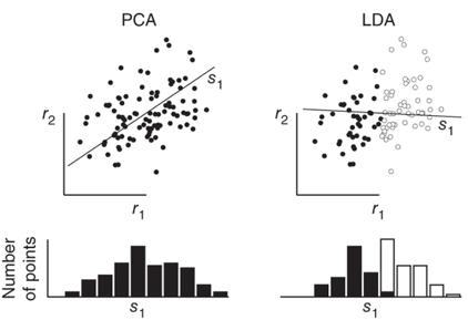
LDA与PCA，LDA与PCA都可以借助SVD求解，但本质是不同的：

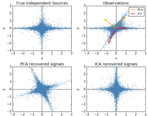
顺便提一句之前梳理的独立成分分析（ICA）与PCA的差别，PCA立足点是相关性，是基于协方差矩阵（二阶统计量）;而ICA立足点是独立性，利用概率分布（也就是高阶统计量），当然如果是正态分布，二者就等价了。

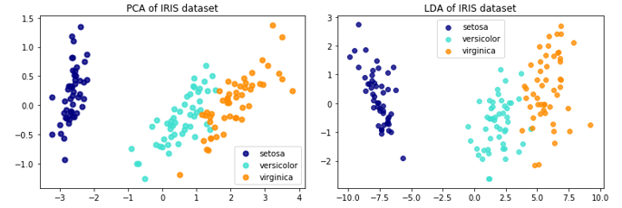
关于LDA、PCA降维的对比，Sklearn给出了IRIS数据的示例：

The Iris dataset represents 3 kind of Iris flowers (Setosa, Versicolour and Virginica) with 4 attributes: sepal length, sepal width, petal length and petal width.即数据类别数是3，每一个样本对应的特征维度是4，现在分别用LDA、PCA降至2维。

code:

print(__doc__)
 
import matplotlib.pyplot as plt
 
from sklearn import datasets
from sklearn.decomposition import PCA
from sklearn.discriminant_analysis import LinearDiscriminantAnalysis
 
iris = datasets.load_iris()
 
X = iris.data
y = iris.target
target_names = iris.target_names
 
pca = PCA(n_components=2)
X_r = pca.fit(X).transform(X)
 
lda = LinearDiscriminantAnalysis(n_components=2)
X_r2 = lda.fit(X, y).transform(X)
 
# Percentage of variance explained for each components
print('explained variance ratio (first two components): %s'
      % str(pca.explained_variance_ratio_))
 
plt.figure()
colors = ['navy', 'turquoise', 'darkorange']
lw = 2
 
for color, i, target_name in zip(colors, [0, 1, 2], target_names):
    plt.scatter(X_r[y == i, 0], X_r[y == i, 1], color=color, alpha=.8, lw=lw,
                label=target_name)
plt.legend(loc='best', shadow=False, scatterpoints=1)
plt.title('PCA of IRIS dataset')
 
plt.figure()
for color, i, target_name in zip(colors, [0, 1, 2], target_names):
    plt.scatter(X_r2[y == i, 0], X_r2[y == i, 1], alpha=.8, color=color,
                label=target_name)
plt.legend(loc='best', shadow=False, scatterpoints=1)
plt.title('LDA of IRIS dataset')
 
plt.show()

Sklearn还提供了归一化：

只在求解方法为lsqr和eigen时有效，就是前面提到的特征值分解和最小二乘啦。

分别用归一化/不归一化：

clf1 = LinearDiscriminantAnalysis(solver='lsqr', shrinkage='auto').fit(X, y)
clf2 = LinearDiscriminantAnalysis(solver='lsqr', shrinkage=None).fit(X, y)

　　应用实例：

from __future__ import division
 
import numpy as np
import matplotlib.pyplot as plt
 
from sklearn.datasets import make_blobs
from sklearn.discriminant_analysis import LinearDiscriminantAnalysis
 
n_train = 20  # samples for training
n_test = 200  # samples for testing
n_averages = 50  # how often to repeat classification
n_features_max = 75  # maximum number of features
step = 4  # step size for the calculation
 
def generate_data(n_samples, n_features):
    """Generate random blob-ish data with noisy features.
 
    This returns an array of input data with shape `(n_samples, n_features)`
    and an array of `n_samples` target labels.
 
    Only one feature contains discriminative information, the other features
    contain only noise.
    """
    X, y = make_blobs(n_samples=n_samples, n_features=1, centers=[[-2], [2]])
 
    # add non-discriminative features
    if n_features > 1:
        X = np.hstack([X, np.random.randn(n_samples, n_features - 1)])
    return X, y
 
acc_clf1, acc_clf2 = [], []
n_features_range = range(1, n_features_max + 1, step)
for n_features in n_features_range:
    score_clf1, score_clf2 = 0, 0
    for _ in range(n_averages):
        X, y = generate_data(n_train, n_features)
 
        clf1 = LinearDiscriminantAnalysis(solver='lsqr', shrinkage='auto').fit(X, y)
        clf2 = LinearDiscriminantAnalysis(solver='lsqr', shrinkage=None).fit(X, y)
 
        X, y = generate_data(n_test, n_features)
        score_clf1 += clf1.score(X, y)
        score_clf2 += clf2.score(X, y)
 
    acc_clf1.append(score_clf1 / n_averages)
    acc_clf2.append(score_clf2 / n_averages)
 
features_samples_ratio = np.array(n_features_range) / n_train
 
plt.plot(features_samples_ratio, acc_clf1, linewidth=2,
         label="Linear Discriminant Analysis with shrinkage", color='navy')
plt.plot(features_samples_ratio, acc_clf2, linewidth=2,
         label="Linear Discriminant Analysis", color='gold')
 
plt.xlabel('n_features / n_samples')
plt.ylabel('Classification accuracy')
 
plt.legend(loc=1, prop={'size': 12})
plt.suptitle('Linear Discriminant Analysis vs. \
shrinkage Linear Discriminant Analysis (1 discriminative feature)')
plt.show()

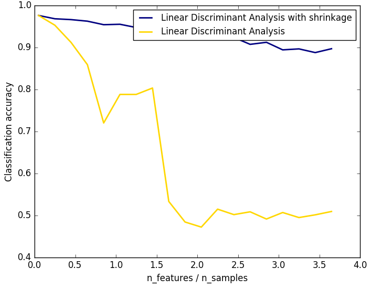
　　结果图可以看出，shrinkage更鲁棒：

参考

• http://blog.csdn.net/daunxx/article/details/51881956
• http://scikit-learn.org/stable/modules/lda_qda.html