t-SNE and PCA

1.t-SNE

知乎

• t-分布领域嵌入算法
• 虽然主打非线性高维数据降维，但是很少用，因为
• 比较适合应用于可视化，测试模型的效果
• 保证在低维上数据的分布与原始特征空间分布的相似性高

因此用来查看分类器的效果更加

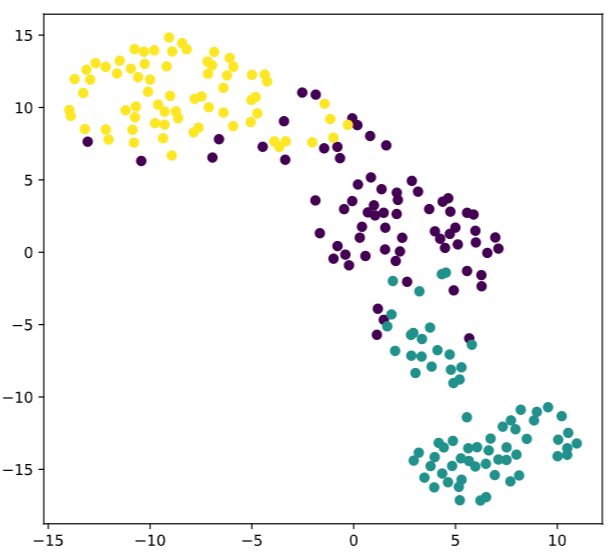
1.1 复现demo

# Import TSNE
from sklearn.manifold import TSNE 
# Create a TSNE instance: model
model = TSNE(learning_rate=200)
# Apply fit_transform to samples: tsne_features
tsne_features = model.fit_transform(samples)
# Select the 0th feature: xs
xs = tsne_features[:,0]
# Select the 1st feature: ys
ys = tsne_features[:,1]
# Scatter plot, coloring by variety_numbers
plt.scatter(xs,ys,c=variety_numbers)
plt.show()

2.PCA

主成分分析是进行特征提取，会在原有的特征的基础上产生新的特征，新特征是原有特征的线性组合，因此会达到降维的目的，但是降维不仅仅只有主成分分析一种

• 当特征变量很多的时候，变量之间往往存在多重共线性。
• 主成分分析,用于高维数据降维，提取数据的主要特征分量
• PCA能“一箭双雕”的地方在于
  • 既可以选择具有代表性的特征，
  • 每个特征之间线性无关
  • 总结一下就是原始特征空间的最佳线性组合
    
    有一个非常易懂的栗子知乎

2.1 数学推理

可以参考【机器学习】降维——PCA（非常详细）

Making sense of principal component analysis, eigenvectors & eigenvalues

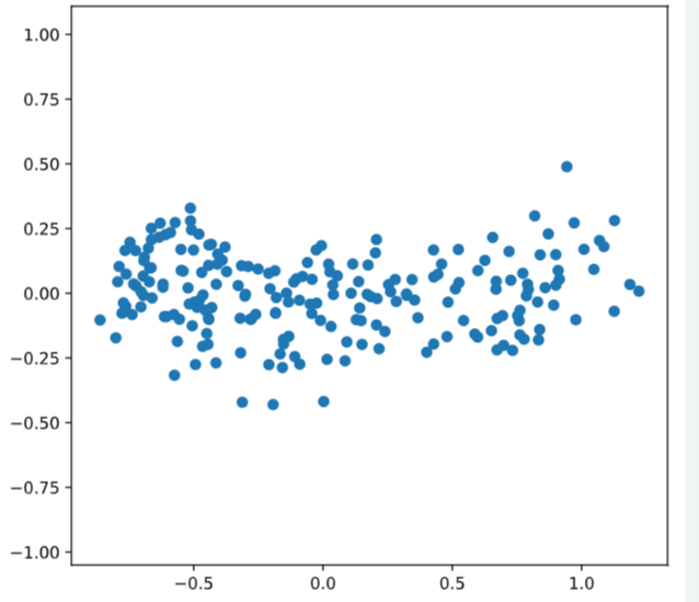
2.2栗子

sklearn里面有直接写好的方法可以直接使用

from sklearn.decomposition import PCA

# Perform the necessary imports
import matplotlib.pyplot as plt
from scipy.stats import pearsonr
# Assign the 0th column of grains: width
width = grains[:,0]
# Assign the 1st column of grains: length
length = grains[:,1]
# Scatter plot width vs length
plt.scatter(width, length)
plt.axis('equal')
plt.show()
# Calculate the Pearson correlation
correlation, pvalue = pearsonr(width, length)
# Display the correlation
print(correlation)

# Import PCA
from sklearn.decomposition import PCA
# Create PCA instance: model
model = PCA()
# Apply the fit_transform method of model to grains: pca_features
pca_features = model.fit_transform(grains)
# Assign 0th column of pca_features: xs
xs = pca_features[:,0]
# Assign 1st column of pca_features: ys
ys = pca_features[:,1]
# Scatter plot xs vs ys
plt.scatter(xs, ys)
plt.axis('equal')
plt.show()
# Calculate the Pearson correlation of xs and ys
correlation, pvalue = pearsonr(xs, ys)
# Display the correlation
print(correlation)
<script.py> output:
    2.5478751053409354e-17

2.3intrinsic dimension

主成分的固有维度，其实就是提取主成分，得到最佳线性组合

2.3.1 提取主成分

.n_components_

提取主成分一般占总的80%以上，不过具体问题还得具体分析

# Perform the necessary imports
from sklearn.decomposition import PCA
from sklearn.preprocessing import StandardScaler
from sklearn.pipeline import make_pipeline
import matplotlib.pyplot as plt
# Create scaler: scaler
scaler = StandardScaler()
# Create a PCA instance: pca
pca = PCA()
# Create pipeline: pipeline
pipeline = make_pipeline(scaler,pca)
# Fit the pipeline to 'samples'
pipeline.fit(samples)
# Plot the explained variances
features =range( pca.n_components_)
plt.bar(features, pca.explained_variance_)
plt.xlabel('PCA feature')
plt.ylabel('variance')
plt.xticks(features)
plt.show()

2.3.2Dimension reduction with PCA

主成分降维

给一个文本特征提取的小例子

虽然我还不知道这个是啥,以后学完补充啊

# Import TfidfVectorizer
from sklearn.feature_extraction.text import TfidfVectorizer
# Create a TfidfVectorizer: tfidf
tfidf = TfidfVectorizer() 
# Apply fit_transform to document: csr_mat
csr_mat = tfidf.fit_transform(documents)
# Print result of toarray() method
print(csr_mat.toarray())
# Get the words: words
words = tfidf.get_feature_names()
# Print words
print(words)
['cats say meow', 'dogs say woof', 'dogs chase cats']
<script.py> output:
    [[0.51785612 0.         0.         0.68091856 0.51785612 0.        ]
     [0.         0.         0.51785612 0.         0.51785612 0.68091856]
     [0.51785612 0.68091856 0.51785612 0.         0.         0.        ]]
    ['cats', 'chase', 'dogs', 'meow', 'say', 'woof']
<script.py> output:
    [[0.51785612 0.         0.         0.68091856 0.51785612 0.        ]
     [0.         0.         0.51785612 0.         0.51785612 0.68091856]
     [0.51785612 0.68091856 0.51785612 0.         0.         0.        ]]
    ['cats', 'chase', 'dogs', 'meow', 'say', 'woof']