课程四(Convolutional Neural Networks),第一周(Foundations of Convolutional Neural Networks) —— 2.Programming assignments:Convolutional Model: step by step
Convolutional Neural Networks: Step by Step
Welcome to Course 4's first assignment! In this assignment, you will implement convolutional (CONV) and pooling (POOL) layers in numpy, including both forward propagation and (optionally) backward propagation.
Notation:
- Superscript [l] denotes an object of the lth layer.
- Example: a[4] is the 4th layer activation. W[5] and b[5] are the 5th layer parameters.
- Superscript (i)denotes an object from the ith example.
- Example: x(i) is the ith training example input.
- Lowerscript i denotes the ith entry of a vector.
- Example: ai[l]denotes the ith entry of the activations in layer l, assuming this is a fully connected (FC) layer.
- nH, nW and nC denote respectively the height, width and number of channels of a given layer. If you want to reference a specific layer l, you can also write nH[l], nW[l], nC[l].
- nHprev, nWprev and nCprev denote respectively the height, width and number of channels of the previous layer. If referencing a specific layer l, this could also be denoted nH[l−1], nW[l−1], nC[l−1].
We assume that you are already familiar with numpy and/or have completed the previous courses of the specialization. Let's get started!
1 - Packages
Let's first import all the packages that you will need during this assignment.
- numpy is the fundamental package for scientific computing with Python.
- matplotlib is a library to plot graphs in Python.
- np.random.seed(1) is used to keep all the random function calls consistent. It will help us grade your work.
【code】
import numpy as np

import h5py

import matplotlib.pyplot as plt

%matplotlib inline

plt.rcParams['figure.figsize'] = (5.0, 4.0) # set default size of plots

plt.rcParams['image.interpolation'] = 'nearest'

plt.rcParams['image.cmap'] = 'gray'

%load_ext autoreload

%autoreload 2

np.random.seed(1)
2 - Outline of the Assignment
You will be implementing the building blocks of a convolutional neural network! Each function you will implement will have detailed instructions that will walk you through the steps needed:
- Convolution functions, including:
- Zero Padding
- Convolve window
- Convolution forward
- Convolution backward (optional)
- Pooling functions, including:
- Pooling forward
- Create mask
- Distribute value
- Pooling backward (optional)
This notebook will ask you to implement these functions from scratch in numpy. In the next notebook, you will use the TensorFlow equivalents of these functions to build the following model:

Note that for every forward function, there is its corresponding backward equivalent. Hence, at every step of your forward module you will store some parameters in a cache. These parameters are used to compute gradients during backpropagation.
【中文翻译】
请注意, 对于每个前向传播, 都有相应的后向传播。因此, 在前向传播模块中的每个步骤中, 您都将在缓存中存储一些参数。这些参数用于在反向传播期间计算导数。
3 - Convolutional Neural Networks
Although programming frameworks make convolutions easy to use, they remain one of the hardest concepts to understand in Deep Learning. A convolution layer transforms an input volume into an output volume of different size, as shown below.
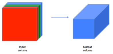
In this part, you will build every step of the convolution layer. You will first implement two helper functions: one for zero padding and the other for computing the convolution function itself.
3.1 - Zero-Padding
Zero-padding adds zeros around the border of an image:

Figure 1 : Zero-Padding
Image (3 channels, RGB) with a padding of 2.
The main benefits of padding are the following:
It allows you to use a CONV layer without necessarily shrinking the height and width of the volumes. This is important for building deeper networks, since otherwise the height/width would shrink as you go to deeper layers. An important special case is the "same" convolution, in which the height/width is exactly preserved after one layer.
It helps us keep more of the information at the border of an image. Without padding, very few values at the next layer would be affected by pixels as the edges of an image.
【中文翻译】
Exercise: Implement the following function, which pads all the images of a batch of examples X with zeros. Use np.pad. Note if you want to pad the array "a" of shape (5,5,5,5,5)(with pad = 1 for the 2nd dimension, pad = 3 for the 4th dimension and pad = 0 for the rest, you would do:
a = np.pad(a, ((0,0), (1,1), (0,0), (3,3), (0,0)), 'constant', constant_values = (..,..))
【code】
# GRADED FUNCTION: zero_pad

def zero_pad(X, pad):

    """

    Pad with zeros all images of the dataset X. The padding is applied to the height and width of an image,

    as illustrated in Figure 1.

    Argument:

    X -- python numpy array of shape (m, n_H, n_W, n_C) representing a batch of m images

    pad -- integer, amount of padding around each image on vertical and horizontal dimensions

    Returns:

    X_pad -- padded image of shape (m, n_H + 2*pad, n_W + 2*pad, n_C)

    """

    ### START CODE HERE ### (≈ 1 line)

    X_pad = np.pad(X,((0,0),(pad,pad),(pad,pad),(0,0)),'constant', constant_values=(0,0) )

    ### END CODE HERE ###

    return X_pad
np.random.seed(1)

x = np.random.randn(4, 3, 3, 2)

x_pad = zero_pad(x, 2)

print ("x.shape =", x.shape)

print ("x_pad.shape =", x_pad.shape)

print ("x[1,1] =", x[1,1])          #编号为1的样本,编号为1的通道

print ("x_pad[1,1] =", x_pad[1,1])

# print ("x=",x) 此处可以打印x,查看x

fig, axarr = plt.subplots(1, 2) # 1行2个窗口

axarr[0].imshow(x[0,:,:,0])  #序号为0,通道为0的样本

axarr[1].set_title('x_pad')

axarr[1].imshow(x_pad[0,:,:,0])  #序号为0,通道为0的样本
【result】
x.shape = (4, 3, 3, 2)

x_pad.shape = (4, 7, 7, 2)

x[1,1] = [[ 0.90085595 -0.68372786]

 [-0.12289023 -0.93576943]

 [-0.26788808  0.53035547]]

x_pad[1,1] = [[ 0.  0.]

 [ 0.  0.]

 [ 0.  0.]

 [ 0.  0.]

 [ 0.  0.]

 [ 0.  0.]

 [ 0.  0.]]
<matplotlib.image.AxesImage at 0x7f94350437f0>
Expected Output:
| x.shape: | (4, 3, 3, 2) |
| x_pad.shape: | (4, 7, 7, 2) |
| x[1,1]: | [[ 0.90085595 -0.68372786] [-0.12289023 -0.93576943] [-0.26788808 0.53035547]] |
| x_pad[1,1]: | [[ 0. 0.] [ 0. 0.] [ 0. 0.] [ 0. 0.] [ 0. 0.] [ 0. 0.] [ 0. 0.]] |
3.2 - Single step of convolution
In this part, implement a single step of convolution, in which you apply the filter to a single position of the input. This will be used to build a convolutional unit, which:
- Takes an input volume
- Applies a filter at every position of the input
- Outputs another volume (usually of different size)

Figure2: Convolution operation
with a filter of 2x2 and a stride of 1 (stride = amount you move the window each time you slide)
In a computer vision application, each value in the matrix on the left corresponds to a single pixel value, and we convolve a 3x3 filter with the image by multiplying its values element-wise with the original matrix, then summing them up and adding a bias. In this first step of the exercise, you will implement a single step of convolution, corresponding to applying a filter to just one of the positions to get a single real-valued output.
Later in this notebook, you'll apply this function to multiple positions of the input to implement the full convolutional operation.
Exercise: Implement conv_single_step(). Hint.
【code】
# GRADED FUNCTION: conv_single_step

def conv_single_step(a_slice_prev, W, b):

    """

    Apply one filter defined by parameters W on a single slice (a_slice_prev) of the output activation

    of the previous layer.

    Arguments:

    a_slice_prev -- slice of input data of shape (f, f, n_C_prev)

    W -- Weight parameters contained in a window - matrix of shape (f, f, n_C_prev)

    b -- Bias parameters contained in a window - matrix of shape (1, 1, 1)

    Returns:

    Z -- a scalar value, result of convolving the sliding window (W, b) on a slice x of the input data

    """

    ### START CODE HERE ### (≈ 2 lines of code)

    # Element-wise product between a_slice and W. Do not add the bias yet.

    s = a_slice_prev * W

    # Sum over all entries of the volume s.

    Z = np.sum(s)

    # Add bias b to Z. Cast b to a float() so that Z results in a scalar value.

    Z = Z + np.float(b)

    ### END CODE HERE ###

    return Z
np.random.seed(1)

a_slice_prev = np.random.randn(4, 4, 3)

W = np.random.randn(4, 4, 3)

b = np.random.randn(1, 1, 1)

Z = conv_single_step(a_slice_prev, W, b)

print("Z =", Z)
【result】
Z = -6.99908945068
Expected Output:
| Z | -6.99908945068 |
3.3 - Convolutional Neural Networks - Forward pass
In the forward pass, you will take many filters and convolve them on the input. Each 'convolution' gives you a 2D matrix output. You will then stack these outputs to get a 3D volume:
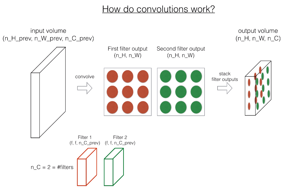
注:原网页是是视频,此处为截图
Exercise: Implement the function below to convolve the filters W on an input activation A_prev. This function takes as input A_prev, the activations output by the previous layer (for a batch of m inputs), F filters/weights denoted by W, and a bias vector denoted by b, where each filter has its own (single) bias. Finally you also have access to the hyperparameters dictionary which contains the stride and the padding.
Hint:
- To select a 2x2 slice at the upper left corner of a matrix "a_prev" (shape (5,5,3)), you would do:
a_slice_prev = a_prev[0:2,0:2,:]
This will be useful when you will define
a_slice_prevbelow, using thestart/endindexes you will define. - To define a_slice you will need to first define its corners
vert_start,vert_end,horiz_startandhoriz_end. This figure may be helpful for you to find how each of the corner can be defined using h, w, f and s in the code below.

Figure 3 : Definition of a slice using vertical and horizontal start/end (with a 2x2 filter)
This figure shows only a single channel.
Reminder: The formulas relating the output shape of the convolution to the input shape is:

For this exercise, we won't worry about vectorization, and will just implement everything with for-loops.
【中文翻译】
练习:实现下面的函数, 在输入激活值 A_prev 上 卷积 过滤器 W。该函数的输入有 :A_prev、前一层的激活值输出 (对于一批 m样本的 输入)、F 过滤器/权重 (W 表示) 和由 b 表示的偏置向量, 其中每个过滤器都有自己的 (单) 偏置。最后, 您还可以访问包含步幅(stride)和填充(padding)的参数字典。
a_slice_prev = a_prev[0:2,0:2,:]

提示: 卷积的输出形状与输入形状之间关系的公式为:

对于这个练习, 我们不会担心矢量化, 只会用 for 循环实现一切。
【code】
# GRADED FUNCTION: conv_forward

def conv_forward(A_prev, W, b, hparameters):

    """

    Implements the forward propagation for a convolution function

    Arguments:

    A_prev -- output activations of the previous layer, numpy array of shape (m, n_H_prev, n_W_prev, n_C_prev)

    W -- Weights, numpy array of shape (f, f, n_C_prev, n_C)

    b -- Biases, numpy array of shape (1, 1, 1, n_C)

    hparameters -- python dictionary containing "stride" and "pad"

    Returns:

    Z -- conv output, numpy array of shape (m, n_H, n_W, n_C)

    cache -- cache of values needed for the conv_backward() function

    """

    ### START CODE HERE ###

    # Retrieve dimensions from A_prev's shape (≈1 line)  从 A_prev 的形状中检索维度

    (m, n_H_prev, n_W_prev, n_C_prev) = A_prev.shape

    # Retrieve dimensions from W's shape (≈1 line)

    (f, f, n_C_prev, n_C) = W.shape

    # Retrieve information from "hparameters" (≈2 lines)

    stride = hparameters["stride"]

    pad =  hparameters["pad"]

    # Compute the dimensions of the CONV output volume using the formula given above. Hint: use int() to floor. (≈2 lines)

    n_H =int((n_H_prev +  2*pad - f)/pad +1)

    n_W =int((n_W_prev +  2*pad - f)/pad +1)

    # Initialize the output volume Z with zeros. (≈1 line)

    Z = np.zeros(((m, n_H, n_W, n_C)))

    # Create A_prev_pad by padding A_prev

    A_prev_pad = zero_pad(A_prev, pad)

    for i in range(m):                               # loop over the batch of training examples

        a_prev_pad = A_prev_pad[i]                   # Select ith training example's padded activation

        for h in range(n_H):                           # loop over vertical axis of the output volume

            for w in range(n_W):                       # loop over horizontal axis of the output volume

                for c in range(n_C):                   # loop over channels (= #filters) of the output volume

                    # Find the corners of the current "slice" (≈4 lines)

                    vert_start = h * stride

                    vert_end = vert_start + f

                    horiz_start = w * stride

                    horiz_end =  w * stride + f

                    # Use the corners to define the (3D) slice of a_prev_pad (See Hint above the cell). (≈1 line)

                    a_slice_prev = a_prev_pad[vert_start: vert_end, horiz_start:horiz_end,:]

                    # Convolve the (3D) slice with the correct filter W and bias b, to get back one output neuron. (≈1 line)

                    Z[i, h, w, c] = conv_single_step(a_slice_prev,W[:,:,:,c],b[:,:,:,c]) #需要找到对应的滤波器,所以 W[:,:,:,c],b[:,:,:,c]

    ### END CODE HERE ###

    # Making sure your output shape is correct

    assert(Z.shape == (m, n_H, n_W, n_C))

    # Save information in "cache" for the backprop

    cache = (A_prev, W, b, hparameters)

    return Z, cache
【result】
Z's mean = 0.0489952035289

Z[3,2,1] = [-0.61490741 -6.7439236  -2.55153897  1.75698377  3.56208902  0.53036437

  5.18531798  8.75898442]

cache_conv[0][1][2][3] = [-0.20075807  0.18656139  0.41005165]
Expected Output:
| Z's mean | 0.0489952035289 |
| Z[3,2,1] | [-0.61490741 -6.7439236 -2.55153897 1.75698377 3.56208902 0.53036437 5.18531798 8.75898442] |
| cache_conv[0][1][2][3] | [-0.20075807 0.18656139 0.41005165] |
Finally, CONV layer should also contain an activation, in which case we would add the following line of code:
# Convolve the window to get back one output neuron

Z[i, h, w, c] = ...

# Apply activation

A[i, h, w, c] = activation(Z[i, h, w, c])
You don't need to do it here.
-------------------------------------------------------------------------------------
【整理者注释:对以下代码块的解释,详见插图】
# Find the corners of the current "slice" (≈4 lines)

                    vert_start = h * stride

                    vert_end = vert_start + f

                    horiz_start = w * stride

                    horiz_end =  w * stride + f

-------------------------------------------------------------------------------------
4 - Pooling layer
The pooling (POOL) layer reduces the height and width of the input. It helps reduce computation, as well as helps make feature detectors more invariant to its position in the input. The two types of pooling layers are:
Max-pooling layer: slides an (f,f) window over the input and stores the max value of the window in the output.
Average-pooling layer: slides an (f,f) window over the input and stores the average value of the window in the output.
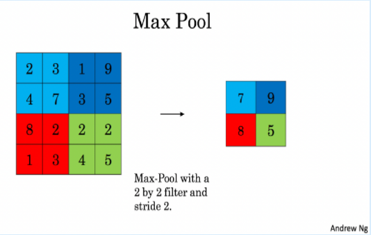
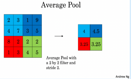
These pooling layers have no parameters for backpropagation to train. However, they have hyperparameters such as the window size f. This specifies the height and width of the fxf window you would compute a max or average over.
【中文翻译】


这些池层没有用于训练的反向传播的参数。然而, 他们有超参数,如窗口大小 f。这将指定要计算最大值或平均值的 fxf 窗口的高度和宽度。
4.1 - Forward Pooling
Now, you are going to implement MAX-POOL and AVG-POOL, in the same function.
Exercise: Implement the forward pass of the pooling layer. Follow the hints in the comments below.
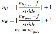
Reminder: As there's no padding, the formulas binding the output shape of the pooling to the input shape is:
【code】
# GRADED FUNCTION: pool_forward

def pool_forward(A_prev, hparameters, mode = "max"):

    """

    Implements the forward pass of the pooling layer

    Arguments:

    A_prev -- Input data, numpy array of shape (m, n_H_prev, n_W_prev, n_C_prev)

    hparameters -- python dictionary containing "f" and "stride"

    mode -- the pooling mode you would like to use, defined as a string ("max" or "average")

    Returns:

    A -- output of the pool layer, a numpy array of shape (m, n_H, n_W, n_C)

    cache -- cache used in the backward pass of the pooling layer, contains the input and hparameters

    """

    # Retrieve dimensions from the input shape

    (m, n_H_prev, n_W_prev, n_C_prev) = A_prev.shape

    # Retrieve hyperparameters from "hparameters"

    f = hparameters["f"]

    stride = hparameters["stride"]

    # Define the dimensions of the output

    n_H = int(1 + (n_H_prev - f) / stride)

    n_W = int(1 + (n_W_prev - f) / stride)

    n_C = n_C_prev

    # Initialize output matrix A

    A = np.zeros((m, n_H, n_W, n_C))

    ### START CODE HERE ###

    for i in range(m):                         # loop over the training examples

        for h in range(n_H):                     # loop on the vertical axis of the output volume

            for w in range(n_W):                 # loop on the horizontal axis of the output volume

                for c in range (n_C):            # loop over the channels of the output volume

                    # Find the corners of the current "slice" (≈4 lines)

                    vert_start = h * stride

                    vert_end =  vert_start + f

                    horiz_start = w * stride

                    horiz_end =  horiz_start + f

                    # Use the corners to define the current slice on the ith training example of A_prev, channel c. (≈1 line)

                    a_prev_slice =  A_prev[i,vert_start: vert_end, horiz_start:horiz_end,c] #此处要对每一个通道取窗口,注意与卷积区别

                    # Compute the pooling operation on the slice. Use an if statment to differentiate the modes. Use np.max/np.mean.

                    if mode == "max":

                        A[i, h, w, c] = np.max(a_prev_slice)

                    elif mode == "average":

                        A[i, h, w, c] = np.mean(a_prev_slice)

    ### END CODE HERE ###

    # Store the input and hparameters in "cache" for pool_backward()

    cache = (A_prev, hparameters)

    # Making sure your output shape is correct

    assert(A.shape == (m, n_H, n_W, n_C))

    return A, cache
np.random.seed(1)

A_prev = np.random.randn(2, 4, 4, 3)

hparameters = {"stride" : 2, "f": 3}

A, cache = pool_forward(A_prev, hparameters)

print("mode = max")

print("A =", A)

print()

A, cache = pool_forward(A_prev, hparameters, mode = "average")

print("mode = average")

print("A =", A)

# print(A.shape) (2,1,1,3)
【result】
mode = max

A = [[[[ 1.74481176  0.86540763  1.13376944]]]

     [[[ 1.13162939  1.51981682  2.18557541]]]]

mode = average

A = [[[[ 0.02105773 -0.20328806 -0.40389855]]]

     [[[-0.22154621  0.51716526  0.48155844]]]]
Expected Output:
| A = | [[[[ 1.74481176 0.86540763 1.13376944]]] [[[ 1.13162939 1.51981682 2.18557541]]]] |
| A = | [[[[ 0.02105773 -0.20328806 -0.40389855]]] [[[-0.22154621 0.51716526 0.48155844]]]] |
Congratulations! You have now implemented the forward passes of all the layers of a convolutional network.
The remainer of this notebook is optional, and will not be graded.
5 - Backpropagation in convolutional neural networks (OPTIONAL / UNGRADED)
In modern deep learning frameworks, you only have to implement the forward pass, and the framework takes care of the backward pass, so most deep learning engineers don't need to bother with the details of the backward pass. The backward pass for convolutional networks is complicated. If you wish however, you can work through this optional portion of the notebook to get a sense of what backprop in a convolutional network looks like.
When in an earlier course you implemented a simple (fully connected) neural network, you used backpropagation to compute the derivatives with respect to the cost to update the parameters. Similarly, in convolutional neural networks you can to calculate the derivatives with respect to the cost in order to update the parameters. The backprop equations are not trivial and we did not derive them in lecture, but we briefly presented them below.
【中文翻译】
5.1 - Convolutional layer backward pass
Let's start by implementing the backward pass for a CONV layer.
5.1.1 - Computing dA:
This is the formula for computing dA with respect to the cost for a certain filter Wc and a given training example:

Where Wc is a filter and dZhw is a scalar corresponding to the gradient of the cost with respect to the output of the conv layer Z at the hth row and wth column (corresponding to the dot product taken at the ith stride left and jth stride down). Note that at each time, we multiply the the same filter Wc by a different dZ when updating dA. We do so mainly because when computing the forward propagation, each filter is dotted and summed by a different a_slice. Therefore when computing the backprop for dA, we are just adding the gradients of all the a_slices.
In code, inside the appropriate for-loops, this formula translates into:
da_prev_pad[vert_start:vert_end, horiz_start:horiz_end, :] += W[:,:,:,c] * dZ[i, h, w, c]
5.1.2 - Computing dW:
This is the formula for computing dWc (dWc is the derivative of one filter) with respect to the loss:

Where aslice corresponds to the slice which was used to generate the acitivation Zij. Hence, this ends up giving us the gradient for W with respect to that slice. Since it is the same W, we will just add up all such gradients to get dW.
In code, inside the appropriate for-loops, this formula translates into:
dW[:,:,:,c] += a_slice * dZ[i, h, w, c]
5.1.3 - Computing db:
This is the formula for computing db with respect to the cost for a certain filter Wc:

As you have previously seen in basic neural networks, db is computed by summing dZ. In this case, you are just summing over all the gradients of the conv output (Z) with respect to the cost.
In code, inside the appropriate for-loops, this formula translates into:
db[:,:,:,c] += dZ[i, h, w, c]
【中文翻译】

其中 Wc 是一个过滤器, dZhw 是一个标量,是成本函数对卷积层输出Z的第h行第w列的值的导数。(对应在第 i 步向左和 第j步向下的点成)。请注意, 每次更新 dA 时, 我们都会用不同的 dZ 乘以相同的过滤器Wc。我们这样做主要是因为在计算正向传播时, 每个过滤器都是用不同的 a_slice 进行点乘和求和的。因此, 当反向传播几算dA时, 我们把所有对 a_slices 的梯度加起来。
在代码中, 在适当的 for 循环内, 此公式转换为:
da_prev_pad[vert_start:vert_end, horiz_start:horiz_end, :] += W[:,:,:,c] * dZ[i, h, w, c]
5.1.2-计算 dWc:
这是计算 dWc(dWc 是一个成本函数对过滤器的导数) 的公式:

dW[:,:,:,c] += a_slice * dZ[i, h, w, c]
5.1.3 - 计算 db:
这是计算 db 的公式(成本函数对某一过滤器Wc ):

db[:,:,:,c] += dZ[i, h, w, c]
Exercise: Implement the conv_backward function below. You should sum over all the training examples, filters, heights, and widths. You should then compute the derivatives using formulas 1, 2 and 3 above.
【code】
def conv_backward(dZ, cache):

    """

    Implement the backward propagation for a convolution function

    Arguments:

    dZ -- gradient of the cost with respect to the output of the conv layer (Z), numpy array of shape (m, n_H, n_W, n_C)

    cache -- cache of values needed for the conv_backward(), output of conv_forward()

    Returns:

    dA_prev -- gradient of the cost with respect to the input of the conv layer (A_prev),

               numpy array of shape (m, n_H_prev, n_W_prev, n_C_prev)

    dW -- gradient of the cost with respect to the weights of the conv layer (W)

          numpy array of shape (f, f, n_C_prev, n_C)

    db -- gradient of the cost with respect to the biases of the conv layer (b)

          numpy array of shape (1, 1, 1, n_C)

    """

    ### START CODE HERE ###

    # Retrieve information from "cache"

    (A_prev, W, b, hparameters) = cache

    # Retrieve dimensions from A_prev's shape

    (m, n_H_prev, n_W_prev, n_C_prev) = A_prev.shape

    # Retrieve dimensions from W's shape

    (f, f, n_C_prev, n_C) = W.shape

    # Retrieve information from "hparameters"

    stride =hparameters["stride"]

    pad = hparameters["pad"]

    # Retrieve dimensions from dZ's shape

    (m, n_H, n_W, n_C) = dZ.shape

    # Initialize dA_prev, dW, db with the correct shapes

    dA_prev = np.random.randn(m, n_H_prev, n_W_prev, n_C_prev)

    dW = np.random.randn(f, f, n_C_prev, n_C)

    db = np.zeros(b.shape)

    # Pad A_prev and dA_prev

    A_prev_pad = zero_pad(A_prev, pad)

    dA_prev_pad =zero_pad(dA_prev, pad)

    for i in range(m):                       # loop over the training examples

        # select ith training example from A_prev_pad and dA_prev_pad

        a_prev_pad =  A_prev_pad[i]

        da_prev_pad = dA_prev_pad[i]

        for h in range(n_H):                   # loop over vertical axis of the output volume

            for w in range(n_W):               # loop over horizontal axis of the output volume

                for c in range(n_C):           # loop over the channels of the output volume

                    # Find the corners of the current "slice"

                    vert_start = h * stride

                    vert_end =  vert_start + f

                    horiz_start = w * stride

                    horiz_end =  horiz_start + f

                    # Use the corners to define the slice from a_prev_pad

                    a_slice = a_prev_pad[vert_start: vert_end, horiz_start:horiz_end,:]

                    # Update gradients for the window and the filter's parameters using the code formulas given above

                    da_prev_pad[vert_start:vert_end, horiz_start:horiz_end, :] +=W[:,:,:,c] * dZ[i, h, w, c]

                    dW[:,:,:,c] += a_slice * dZ[i, h, w, c]

                    db[:,:,:,c] += dZ[i, h, w, c]

        # Set the ith training example's dA_prev to the unpaded da_prev_pad (Hint: use X[pad:-pad, pad:-pad, :])

        dA_prev[i, :, :, :] =dA_prev_pad[i,pad:-pad, pad:-pad, :]

    ### END CODE HERE ###

    # Making sure your output shape is correct

    assert(dA_prev.shape == (m, n_H_prev, n_W_prev, n_C_prev))

    return dA_prev, dW, db
np.random.seed(1)

dA, dW, db = conv_backward(Z, cache_conv) #此处传入的为什么是Z,而不是dZ  ???

print("dA_mean =", np.mean(dA))

print("dW_mean =", np.mean(dW))

print("db_mean =", np.mean(db))
【result】
dA_mean = 1.50871418576

dW_mean = 1.80043206846

db_mean = 7.83923256462
Expected Output:
dA_mean    1.45243777754

dW_mean    1.72699145831

db_mean    7.83923256462
-------------------------------------------------------------------------------------
【整理者注释:解释以下代码】
 # Set the ith training example's dA_prev to the unpaded da_prev_pad (Hint: use X[pad:-pad, pad:-pad, :])

        dA_prev[i, :, :, :] =dA_prev_pad[i,pad:-pad, pad:-pad, :]
【问题】:为什么  dA_prev[i, :, :, :] =dA_prev_pad[i,pad:-pad, pad:-pad, :] ?

【用代码验证如下】
# (n_H,n_W,n_C)=(1,1,2)

a=np.array([[[1,2]]])   #临时造的数据

print("a.shape=",a.shape)
a.shape= (1, 1, 2)
# 进行pad操作,pad=1, 则(n_H_pad,n_W_pad,n_C_pad)=(3,3,2)

b=np.array([[[1,2],[3,4],[3,4]],[[7,8],[1,2],[3,4]],[[7,8],[1,2],[3,4]]]) #临时造的数据

print("b.shape=",b.shape)
b.shape= (3, 3, 2)
# 验证 b[pad:-pad, pad:-pad, :] 的shape是否与a的shape一致

pad=1

c=b[pad:-pad, pad:-pad, :]

print("c.shape=",c.shape)

assert(a.shape==c.shape)

#运行结果没有报错,所以 b[pad:-pad, pad:-pad, :] 的shape是否与a的shape一致

#从运行结果上也可以看出,shape都为(1,1,2)
c.shape= (1, 1, 2)
print("a=",a)

print("c=",c)     #a和c是一样的
a= [[[1 2]]]

c= [[[1 2]]]
-------------------------------------------------------------------------------------
5.2 Pooling layer - backward pass
Next, let's implement the backward pass for the pooling layer, starting with the MAX-POOL layer. Even though a pooling layer has no parameters for backprop to update, you still need to backpropagation the gradient through the pooling layer in order to compute gradients for layers that came before the pooling layer.
5.2.1 Max pooling - backward pass
Before jumping into the backpropagation of the pooling layer, you are going to build a helper function called create_mask_from_window() which does the following:

As you can see, this function creates a "mask" matrix which keeps track of where the maximum of the matrix is. True (1) indicates the position of the maximum in X, the other entries are False (0). You'll see later that the backward pass for average pooling will be similar to this but using a different mask.
Exercise: Implement create_mask_from_window(). This function will be helpful for pooling backward. Hints:
- np.max() may be helpful. It computes the maximum of an array.
- If you have a matrix X and a scalar x:
A = (X == x)will return a matrix A of the same size as X such that:A[i,j] = True if X[i,j] = x
A[i,j] = False if X[i,j] != x
- Here, you don't need to consider cases where there are several maxima in a matrix.
【code】
def create_mask_from_window(x):

    """

    Creates a mask from an input matrix x, to identify the max entry of x.

    Arguments:

    x -- Array of shape (f, f)

    Returns:

    mask -- Array of the same shape as window, contains a True at the position corresponding to the max entry of x.

    """

    ### START CODE HERE ### (≈1 line)

    mask = (x == np.max(x))

    ### END CODE HERE ###

    return mask
np.random.seed(1)

x = np.random.randn(2,3)

mask = create_mask_from_window(x)

print('x = ', x)

print("mask = ", mask)
【result】
x =  [[ 1.62434536 -0.61175641 -0.52817175]

 [-1.07296862  0.86540763 -2.3015387 ]]

mask =  [[ True False False]

 [False False False]]
Expected Output:
x =    [[ 1.62434536 -0.61175641 -0.52817175]

        [-1.07296862  0.86540763 -2.3015387 ]]

mask =    [[ True False False]

           [False False False]]
Why do we keep track of the position of the max? It's because this is the input value that ultimately influenced the output, and therefore the cost. Backprop is computing gradients with respect to the cost, so anything that influences the ultimate cost should have a non-zero gradient. So, backprop will "propagate" the gradient back to this particular input value that had influenced the cost.
5.2.2 - Average pooling - backward pass
In max pooling, for each input window, all the "influence" on the output came from a single input value--the max. In average pooling, every element of the input window has equal influence on the output. So to implement backprop, you will now implement a helper function that reflects this.
For example if we did average pooling in the forward pass using a 2x2 filter, then the mask you'll use for the backward pass will look like:

This implies that each position in the dZ matrix contributes equally to output because in the forward pass, we took an average.
Exercise: Implement the function below to equally distribute a value dz through a matrix of dimension shape. Hint
【code】
def distribute_value(dz, shape):

    """

    Distributes the input value in the matrix of dimension shape

    Arguments:

    dz -- input scalar

    shape -- the shape (n_H, n_W) of the output matrix for which we want to distribute the value of dz

    Returns:

    a -- Array of size (n_H, n_W) for which we distributed the value of dz

    """

    ### START CODE HERE ###

    # Retrieve dimensions from shape (≈1 line)

    (n_H, n_W) = shape

    # Compute the value to distribute on the matrix (≈1 line)

    average = dz/(n_H * n_W)

    # Create a matrix where every entry is the "average" value (≈1 line)

    a = np.ones( (n_H, n_W))*average

    ### END CODE HERE ###

    return a
a = distribute_value(2, (2,2))

print('distributed value =', a)
【result】
distributed value = [[ 0.5  0.5]

                     [ 0.5  0.5]]
Expected Output:
distributed_value =    [[ 0.5 0.5]

                        [ 0.5 0.5]]
5.2.3 Putting it together: Pooling backward
You now have everything you need to compute backward propagation on a pooling layer.
Exercise: Implement the pool_backward function in both modes ("max" and "average"). You will once again use 4 for-loops (iterating over training examples, height, width, and channels). You should use an if/elif statement to see if the mode is equal to 'max' or 'average'. If it is equal to 'average' you should use the distribute_value() function you implemented above to create a matrix of the same shape as a_slice. Otherwise, the mode is equal to 'max', and you will create a mask with create_mask_from_window() and multiply it by the corresponding value of dZ.
【code】
def pool_backward(dA, cache, mode = "max"):

    """

    Implements the backward pass of the pooling layer

    Arguments:

    dA -- gradient of cost with respect to the output of the pooling layer, same shape as A

    cache -- cache output from the forward pass of the pooling layer, contains the layer's input and hparameters

    mode -- the pooling mode you would like to use, defined as a string ("max" or "average")

    Returns:

    dA_prev -- gradient of cost with respect to the input of the pooling layer, same shape as A_prev

    """

    ### START CODE HERE ###

    # Retrieve information from cache (≈1 line)

    (A_prev, hparameters) = cache

    # Retrieve hyperparameters from "hparameters" (≈2 lines)

    stride = hparameters["stride"]

    f = hparameters["f"]

    # Retrieve dimensions from A_prev's shape and dA's shape (≈2 lines)

    m, n_H_prev, n_W_prev, n_C_prev = A_prev.shape

    m, n_H, n_W, n_C = dA.shape

    # Initialize dA_prev with zeros (≈1 line)

    dA_prev = np.zeros( A_prev.shape)

    for i in range(m):                       # loop over the training examples

        # select training example from A_prev (≈1 line)

        a_prev = A_prev[i]

        for h in range(n_H):                   # loop on the vertical axis

            for w in range(n_W):               # loop on the horizontal axis

                for c in range(n_C):           # loop over the channels (depth)

                    # Find the corners of the current "slice" (≈4 lines)

                    vert_start = h*stride

                    vert_end = h*stride + f

                    horiz_start = w *stride

                    horiz_end =w *stride  + f

                    # Compute the backward propagation in both modes.

                    if mode == "max":

                        # Use the corners and "c" to define the current slice from a_prev (≈1 line)

                        a_prev_slice =  a_prev[ vert_start:vert_end, horiz_start: horiz_end,c]

                        # Create the mask from a_prev_slice (≈1 line)

                        mask =  create_mask_from_window( a_prev_slice )

                        # Set dA_prev to be dA_prev + (the mask multiplied by the correct entry of dA) (≈1 line)

                        dA_prev[i, vert_start: vert_end, horiz_start: horiz_end, c] +=  mask*dA[i,h,w,c]

                    elif mode == "average":

                        # Get the value a from dA (≈1 line)

                        da = dA[i,h,w,c]

                        # Define the shape of the filter as fxf (≈1 line)

                        shape = (f,f)

                        # Distribute it to get the correct slice of dA_prev. i.e. Add the distributed value of da. (≈1 line)

                        dA_prev[i, vert_start: vert_end, horiz_start: horiz_end, c] += distribute_value(da, shape)

    ### END CODE ###

    # Making sure your output shape is correct

    assert(dA_prev.shape == A_prev.shape)

    return dA_prev
np.random.seed(1)

A_prev = np.random.randn(5, 5, 3, 2)

hparameters = {"stride" : 1, "f": 2}

A, cache = pool_forward(A_prev, hparameters)

dA = np.random.randn(5, 4, 2, 2)

dA_prev = pool_backward(dA, cache, mode = "max")

print("mode = max")

print('mean of dA = ', np.mean(dA))

print('dA_prev[1,1] = ', dA_prev[1,1])

print()

dA_prev = pool_backward(dA, cache, mode = "average")

print("mode = average")

print('mean of dA = ', np.mean(dA))

print('dA_prev[1,1] = ', dA_prev[1,1])
【result】
mode = max

mean of dA =  0.145713902729

dA_prev[1,1] =  [[ 0.          0.        ]

 [ 5.05844394 -1.68282702]

 [ 0.          0.        ]]

mode = average

mean of dA =  0.145713902729

dA_prev[1,1] =  [[ 0.08485462  0.2787552 ]

 [ 1.26461098 -0.25749373]

 [ 1.17975636 -0.53624893]]
Expected Output:
mode = max:

mean of dA =    0.145713902729

dA_prev[1,1] =    [[ 0. 0. ]

[ 5.05844394 -1.68282702]

[ 0. 0. ]]

mode = average

mean of dA =    0.145713902729

dA_prev[1,1] =    [[ 0.08485462 0.2787552 ]

[ 1.26461098 -0.25749373]

[ 1.17975636 -0.53624893]]
Congratulations !
Congratulation on completing this assignment. You now understand how convolutional neural networks work. You have implemented all the building blocks of a neural network. In the next assignment you will implement a ConvNet using TensorFlow.
课程四(Convolutional Neural Networks),第一周(Foundations of Convolutional Neural Networks) —— 2.Programming assignments:Convolutional Model: step by step的更多相关文章
- 课程五(Sequence Models),第一 周(Recurrent Neural Networks) —— 1.Programming assignments:Building a recurrent neural network - step by step
Building your Recurrent Neural Network - Step by Step Welcome to Course 5's first assignment! In thi ...
- 课程五(Sequence Models),第一 周(Recurrent Neural Networks) —— 2.Programming assignments:Dinosaur Island - Character-Level Language Modeling
Character level language model - Dinosaurus land Welcome to Dinosaurus Island! 65 million years ago, ...
- 课程五(Sequence Models),第一 周(Recurrent Neural Networks) —— 3.Programming assignments:Jazz improvisation with LSTM
Improvise a Jazz Solo with an LSTM Network Welcome to your final programming assignment of this week ...
- 课程五(Sequence Models),第一 周(Recurrent Neural Networks) —— 0.Practice questions:Recurrent Neural Networks
[解释] It is appropriate when every input should be matched to an output. [解释] in a language model we ...
- 课程四(Convolutional Neural Networks),第一周(Foundations of Convolutional Neural Networks) —— 3.Programming assignments:Convolutional Model: application
Convolutional Neural Networks: Application Welcome to Course 4's second assignment! In this notebook ...
- 课程四(Convolutional Neural Networks),第四 周(Special applications: Face recognition & Neural style transfer) —— 3.Programming assignments:Face Recognition for the Happy House
Face Recognition for the Happy House Welcome to the first assignment of week 4! Here you will build ...
- 吴恩达《深度学习》-第五门课 序列模型(Sequence Models)-第一周 循环序列模型(Recurrent Neural Networks) -课程笔记
第一周 循环序列模型(Recurrent Neural Networks) 1.1 为什么选择序列模型?(Why Sequence Models?) 1.2 数学符号(Notation) 这个输入数据 ...
- 吴恩达《深度学习》-第二门课 (Improving Deep Neural Networks:Hyperparameter tuning, Regularization and Optimization)-第一周:深度学习的实践层面 (Practical aspects of Deep Learning) -课程笔记
第一周:深度学习的实践层面 (Practical aspects of Deep Learning) 1.1 训练,验证,测试集(Train / Dev / Test sets) 创建新应用的过程中, ...
- 吴恩达《深度学习》-课后测验-第二门课 (Improving Deep Neural Networks:Hyperparameter tuning, Regularization and Optimization)-Week 1 - Practical aspects of deep learning(第一周测验 - 深度学习的实践)
Week 1 Quiz - Practical aspects of deep learning(第一周测验 - 深度学习的实践) \1. If you have 10,000,000 example ...
随机推荐
- python狂犬病大数据分析
一.被动物咬伤.抓伤者,年龄以45-59岁年龄组为最多(占30.66%). 45-59岁年龄段的人与动物接触较多.被侵害的机会最多.其次受伤机会较多的是15-44岁年龄阶段的人,而7岁及以下儿童受伤比 ...
- Scanner 随机数
import java.util.Scanner; import java.util.Scanner; Sc ...
- 基于ASP.NET高职学生工作管理系统--文献随笔(八)
一.基本信息 标题:基于ASP.NET高职学生工作管理系统 时间:2015 出版源:电子科技大学 关键词:高职; 学生管理; ASP.NET; 系统; 二.研究背景 问题定义:随着社会的发展,我国经济 ...
- 查看class实际执行的类路径
查看class真实归属的jar包位置getClass().getClassLoader().getResource(getClass().getName().replace('.', '/') + & ...
- python_paramiko
目录: paramiko模块介绍 paramiko模块安装 paramiko模块使用 一.paramiko模块介绍 paramiko是一个用于做远程控制的模块,使用该模块可以对远程服务器进行命令或文件 ...
- 结合OPENSIFT源码详解SIFT算法
平台:win10 x64 +VS 2015专业版 +opencv-2.4.11 + gtk_-bundle_2.24.10_win32 参考博客:https://www.cnblogs.com/cql ...
- CQOI2018 简要题解
破解D-H协议 列个式子会发现是BSGSBSGSBSGS的模板题,直接码就是了. 代码: #include<bits/stdc++.h> #include<tr1/unordered ...
- Solidity合约记录——(三)如何在合约中对操作进行权限控制
合约中一般会有多种针对不同数据的操作:例如对于存证内容的增加.更新及查询,若不进行一套符合要求的权限控制,事实上整个合约在真实环境下是没有多少使用价值的.那么应当如何对合约的权限进行划分?我们针对So ...
- wx:for类表渲染
列表渲染 wx:for 在组件上使用wx:for控制属性绑定一个数组,即可使用数组中各项的数据重复渲染该组件. 默认数组的当前项的下标变量名默认为index,数组当前项的变量名默认为item < ...
- tarjan求强连通分量+缩点+割点/割桥(点双/边双)以及一些证明
“tarjan陪伴强联通分量 生成树完成后思路才闪光 欧拉跑过的七桥古塘 让你 心驰神往”----<膜你抄> 自从听完这首歌,我就对tarjan开始心驰神往了,不过由于之前水平不足,一 ...
