tensorflow神经网络拟合非线性函数与操作指南
本实验通过建立一个含有两个隐含层的BP神经网络,拟合具有二次函数非线性关系的方程,并通过可视化展现学习到的拟合曲线,同时随机给定输入值,输出预测值,最后给出一些关键的提示。
源代码如下:
- # -*- coding: utf-8 -*-
- import tensorflow as tf
- import numpy as np
- import matplotlib.pyplot as plt
- plotdata = { "batchsize":[], "loss":[] }
- def moving_average(a, w=11):
- if len(a) < w:
- return a[:]
- return [val if idx < w else sum(a[(idx-w):idx])/w for idx, val in enumerate(a)]
- #生成模拟数据,二次函数关系
- train_X = np.linspace(-1, 1, 100)[:, np.newaxis]
- train_Y = train_X*train_X + 5 * train_X + np.random.randn(*train_X.shape) * 0.3
- #子图1显示模拟数据点
- plt.figure(12)
- plt.subplot(221)
- plt.plot(train_X, train_Y, 'ro', label='Original data')
- plt.legend()
- # 创建模型
- # 占位符
- X = tf.placeholder("float",[None,1])
- Y = tf.placeholder("float",[None,1])
- # 模型参数
- W1 = tf.Variable(tf.random_normal([1,10]), name="weight1")
- b1 = tf.Variable(tf.zeros([1,10]), name="bias1")
- W2 = tf.Variable(tf.random_normal([10,6]), name="weight2")
- b2 = tf.Variable(tf.zeros([1,6]), name="bias2")
- W3 = tf.Variable(tf.random_normal([6,1]), name="weight3")
- b3 = tf.Variable(tf.zeros([1]), name="bias3")
- # 前向结构
- z1 = tf.matmul(X, W1) + b1
- z2 = tf.nn.relu(z1)
- z3 = tf.matmul(z2, W2) + b2
- z4 = tf.nn.relu(z3)
- z5 = tf.matmul(z4, W3) + b3
- #反向优化
- cost =tf.reduce_mean( tf.square(Y - z5))
- learning_rate = 0.01
- optimizer = tf.train.GradientDescentOptimizer(learning_rate).minimize(cost) #Gradient descent
- # 初始化变量
- init = tf.global_variables_initializer()
- # 训练参数
- training_epochs = 5000
- display_step = 2
- # 启动session
- with tf.Session() as sess:
- sess.run(init)
- for epoch in range(training_epochs+1):
- sess.run(optimizer, feed_dict={X: train_X, Y: train_Y})
- #显示训练中的详细信息
- if epoch % display_step == 0:
- loss = sess.run(cost, feed_dict={X: train_X, Y:train_Y})
- print ("Epoch:", epoch, "cost=", loss)
- if not (loss == "NA" ):
- plotdata["batchsize"].append(epoch)
- plotdata["loss"].append(loss)
- print (" Finish")
- #图形显示
- plt.subplot(222)
- plt.plot(train_X, train_Y, 'ro', label='Original data')
- plt.plot(train_X, sess.run(z5, feed_dict={X: train_X}), label='Fitted line')
- plt.legend()
- plotdata["avgloss"] = moving_average(plotdata["loss"])
- plt.subplot(212)
- plt.plot(plotdata["batchsize"], plotdata["avgloss"], 'b--')
- plt.xlabel('Minibatch number')
- plt.ylabel('Loss')
- plt.title('Minibatch run vs Training loss')
- plt.show()
- #预测结果
- a=[[0.2],[0.3]]
- print ("x=[[0.2],[0.3]],z5=", sess.run(z5, feed_dict={X: a}))
运行结果如下:
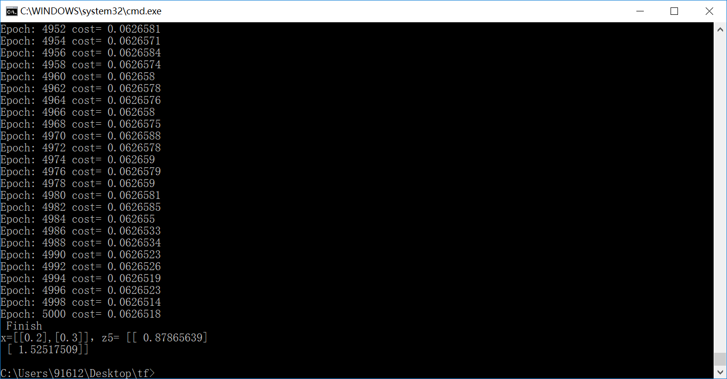
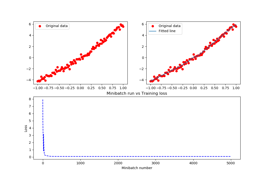
结果实在是太棒了,把这个关系拟合的非常好。在上述的例子中,需要进一步说明如下内容:
- 输入节点可以通过字典类型定义,而后通过字典的方法访问
- input = {
- 'X': tf.placeholder("float",[None,1]),
- 'Y': tf.placeholder("float",[None,1])
- }
sess.run(optimizer, feed_dict={input['X']: train_X, input['Y']: train_Y})
直接定义输入节点的方法是不推荐使用的。
- 变量也可以通过字典类型定义,例如上述代码可以改为:
- parameter = {
- 'W1': tf.Variable(tf.random_normal([1,10]), name="weight1"),
- 'b1': tf.Variable(tf.zeros([1,10]), name="bias1"),
- 'W2': tf.Variable(tf.random_normal([10,6]), name="weight2"),
- 'b2': tf.Variable(tf.zeros([1,6]), name="bias2"),
- 'W3': tf.Variable(tf.random_normal([6,1]), name="weight3"),
- 'b3': tf.Variable(tf.zeros([1]), name="bias3")
- }
- z1 = tf.matmul(X, parameter['W1']) +parameter['b1']
在上述代码中练习保存/载入模型,代码如下:
- # -*- coding: utf-8 -*-
- import tensorflow as tf
- import numpy as np
- import matplotlib.pyplot as plt
- plotdata = { "batchsize":[], "loss":[] }
- def moving_average(a, w=11):
- if len(a) < w:
- return a[:]
- return [val if idx < w else sum(a[(idx-w):idx])/w for idx, val in enumerate(a)]
- #生成模拟数据,二次函数关系
- train_X = np.linspace(-1, 1, 100)[:, np.newaxis]
- train_Y = train_X*train_X + 5 * train_X + np.random.randn(*train_X.shape) * 0.3
- #子图1显示模拟数据点
- plt.figure(12)
- plt.subplot(221)
- plt.plot(train_X, train_Y, 'ro', label='Original data')
- plt.legend()
- # 创建模型
- # 字典型占位符
- input = {'X':tf.placeholder("float",[None,1]),
- 'Y':tf.placeholder("float",[None,1])}
- # X = tf.placeholder("float",[None,1])
- # Y = tf.placeholder("float",[None,1])
- # 模型参数
- parameter = {'W1':tf.Variable(tf.random_normal([1,10]), name="weight1"), 'b1':tf.Variable(tf.zeros([1,10]), name="bias1"),
- 'W2':tf.Variable(tf.random_normal([10,6]), name="weight2"),'b2':tf.Variable(tf.zeros([1,6]), name="bias2"),
- 'W3':tf.Variable(tf.random_normal([6,1]), name="weight3"), 'b3':tf.Variable(tf.zeros([1]), name="bias3")}
- # W1 = tf.Variable(tf.random_normal([1,10]), name="weight1")
- # b1 = tf.Variable(tf.zeros([1,10]), name="bias1")
- # W2 = tf.Variable(tf.random_normal([10,6]), name="weight2")
- # b2 = tf.Variable(tf.zeros([1,6]), name="bias2")
- # W3 = tf.Variable(tf.random_normal([6,1]), name="weight3")
- # b3 = tf.Variable(tf.zeros([1]), name="bias3")
- # 前向结构
- z1 = tf.matmul(input['X'], parameter['W1']) + parameter['b1']
- z2 = tf.nn.relu(z1)
- z3 = tf.matmul(z2, parameter['W2']) + parameter['b2']
- z4 = tf.nn.relu(z3)
- z5 = tf.matmul(z4, parameter['W3']) + parameter['b3']
- #反向优化
- cost =tf.reduce_mean( tf.square(input['Y'] - z5))
- learning_rate = 0.01
- optimizer = tf.train.GradientDescentOptimizer(learning_rate).minimize(cost) #Gradient descent
- # 初始化变量
- init = tf.global_variables_initializer()
- # 训练参数
- training_epochs = 5000
- display_step = 2
- # 生成saver
- saver = tf.train.Saver()
- savedir = "model/"
- # 启动session
- with tf.Session() as sess:
- sess.run(init)
- for epoch in range(training_epochs+1):
- sess.run(optimizer, feed_dict={input['X']: train_X, input['Y']: train_Y})
- #显示训练中的详细信息
- if epoch % display_step == 0:
- loss = sess.run(cost, feed_dict={input['X']: train_X, input['Y']:train_Y})
- print ("Epoch:", epoch, "cost=", loss)
- if not (loss == "NA" ):
- plotdata["batchsize"].append(epoch)
- plotdata["loss"].append(loss)
- print (" Finish")
- #保存模型
- saver.save(sess, savedir+"mymodel.cpkt")
- #图形显示
- plt.subplot(222)
- plt.plot(train_X, train_Y, 'ro', label='Original data')
- plt.plot(train_X, sess.run(z5, feed_dict={input['X']: train_X}), label='Fitted line')
- plt.legend()
- plotdata["avgloss"] = moving_average(plotdata["loss"])
- plt.subplot(212)
- plt.plot(plotdata["batchsize"], plotdata["avgloss"], 'b--')
- plt.xlabel('Minibatch number')
- plt.ylabel('Loss')
- plt.title('Minibatch run vs Training loss')
- plt.show()
- #预测结果
- #在另外一个session里面载入保存的模型,再测试
- a=[[0.2],[0.3]]
- with tf.Session() as sess2:
- #sess2.run(tf.global_variables_initializer())可有可无,因为下面restore会载入参数,相当于本次调用的初始化
- saver.restore(sess2, "model/mymodel.cpkt")
- print ("x=[[0.2],[0.3]],z5=", sess2.run(z5, feed_dict={input['X']: a}))
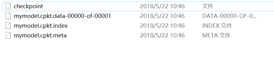
生成如下目录:
上述代码模型的载入没有利用到检查点文件,显得不够智能,还需用户去查找指定某一模型,那在很多算法项目中是不需要用户去找的,而可以通过检查点找到保存的模型。例如:
- # -*- coding: utf-8 -*-
- import tensorflow as tf
- import numpy as np
- import matplotlib.pyplot as plt
- plotdata = { "batchsize":[], "loss":[] }
- def moving_average(a, w=11):
- if len(a) < w:
- return a[:]
- return [val if idx < w else sum(a[(idx-w):idx])/w for idx, val in enumerate(a)]
- #生成模拟数据,二次函数关系
- train_X = np.linspace(-1, 1, 100)[:, np.newaxis]
- train_Y = train_X*train_X + 5 * train_X + np.random.randn(*train_X.shape) * 0.3
- #子图1显示模拟数据点
- plt.figure(12)
- plt.subplot(221)
- plt.plot(train_X, train_Y, 'ro', label='Original data')
- plt.legend()
- # 创建模型
- # 字典型占位符
- input = {'X':tf.placeholder("float",[None,1]),
- 'Y':tf.placeholder("float",[None,1])}
- # X = tf.placeholder("float",[None,1])
- # Y = tf.placeholder("float",[None,1])
- # 模型参数
- parameter = {'W1':tf.Variable(tf.random_normal([1,10]), name="weight1"), 'b1':tf.Variable(tf.zeros([1,10]), name="bias1"),
- 'W2':tf.Variable(tf.random_normal([10,6]), name="weight2"),'b2':tf.Variable(tf.zeros([1,6]), name="bias2"),
- 'W3':tf.Variable(tf.random_normal([6,1]), name="weight3"), 'b3':tf.Variable(tf.zeros([1]), name="bias3")}
- # W1 = tf.Variable(tf.random_normal([1,10]), name="weight1")
- # b1 = tf.Variable(tf.zeros([1,10]), name="bias1")
- # W2 = tf.Variable(tf.random_normal([10,6]), name="weight2")
- # b2 = tf.Variable(tf.zeros([1,6]), name="bias2")
- # W3 = tf.Variable(tf.random_normal([6,1]), name="weight3")
- # b3 = tf.Variable(tf.zeros([1]), name="bias3")
- # 前向结构
- z1 = tf.matmul(input['X'], parameter['W1']) + parameter['b1']
- z2 = tf.nn.relu(z1)
- z3 = tf.matmul(z2, parameter['W2']) + parameter['b2']
- z4 = tf.nn.relu(z3)
- z5 = tf.matmul(z4, parameter['W3']) + parameter['b3']
- #反向优化
- cost =tf.reduce_mean( tf.square(input['Y'] - z5))
- learning_rate = 0.01
- optimizer = tf.train.GradientDescentOptimizer(learning_rate).minimize(cost) #Gradient descent
- # 初始化变量
- init = tf.global_variables_initializer()
- # 训练参数
- training_epochs = 5000
- display_step = 2
- # 生成saver
- saver = tf.train.Saver(max_to_keep=1)
- savedir = "model/"
- # 启动session
- with tf.Session() as sess:
- sess.run(init)
- for epoch in range(training_epochs+1):
- sess.run(optimizer, feed_dict={input['X']: train_X, input['Y']: train_Y})
- saver.save(sess, savedir+"mymodel.cpkt",global_step=epoch)
- #显示训练中的详细信息
- if epoch % display_step == 0:
- loss = sess.run(cost, feed_dict={input['X']: train_X, input['Y']:train_Y})
- print ("Epoch:", epoch, "cost=", loss)
- if not (loss == "NA" ):
- plotdata["batchsize"].append(epoch)
- plotdata["loss"].append(loss)
- print (" Finish")
- #图形显示
- plt.subplot(222)
- plt.plot(train_X, train_Y, 'ro', label='Original data')
- plt.plot(train_X, sess.run(z5, feed_dict={input['X']: train_X}), label='Fitted line')
- plt.legend()
- plotdata["avgloss"] = moving_average(plotdata["loss"])
- plt.subplot(212)
- plt.plot(plotdata["batchsize"], plotdata["avgloss"], 'b--')
- plt.xlabel('Minibatch number')
- plt.ylabel('Loss')
- plt.title('Minibatch run vs Training loss')
- plt.show()
- #预测结果
- #在另外一个session里面载入保存的模型,再测试
- a=[[0.2],[0.3]]
- load=5000
- with tf.Session() as sess2:
- #sess2.run(tf.global_variables_initializer())可有可无,因为下面restore会载入参数,相当于本次调用的初始化
- #saver.restore(sess2, "model/mymodel.cpkt")
- saver.restore(sess2, "model/mymodel.cpkt-" + str(load))
- print ("x=[[0.2],[0.3]],z5=", sess2.run(z5, feed_dict={input['X']: a}))
- #通过检查点文件载入保存的模型
- with tf.Session() as sess3:
- ckpt = tf.train.get_checkpoint_state(savedir)
- if ckpt and ckpt.model_checkpoint_path:
- saver.restore(sess3, ckpt.model_checkpoint_path)
- print ("x=[[0.2],[0.3]],z5=", sess3.run(z5, feed_dict={input['X']: a}))
- #通过检查点文件载入最新保存的模型
- with tf.Session() as sess4:
- ckpt = tf.train.latest_checkpoint(savedir)
- if ckpt!=None:
- saver.restore(sess4, ckpt)
- print ("x=[[0.2],[0.3]],z5=", sess4.run(z5, feed_dict={input['X']: a}))
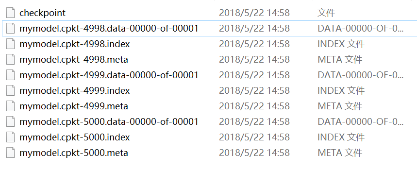
而通常情况下,上述两种通过检查点载入模型参数的结果是一样的,主要是因为不管用户保存了多少个模型文件,都会被记录在唯一一个检查点文件中,这个指定保存模型个数的参数就是max_to_keep,例如:
- saver = tf.train.Saver(max_to_keep=3)
而检查点都会默认用最新的模型载入,忽略了之前的模型,因此上述两个检查点载入了同一个模型,自然最后输出的测试结果是一致的。保存的三个模型如图:
接下来,为什么上面的变量,需要给它对应的操作起个名字,而且是不一样的名字呢?像weight1、bias1等等。大家都知道,名字这个东西太重要了,通过它可以访问我们想访问的变量,也就可以对其进行一些操作。例如:
- 显示模型的内容
不同版本的函数会有些区别,本文试验的版本是1.7.0,代码例如:
- # -*- coding: utf-8 -*-
- import tensorflow as tf
- from tensorflow.python.tools import inspect_checkpoint as chkp
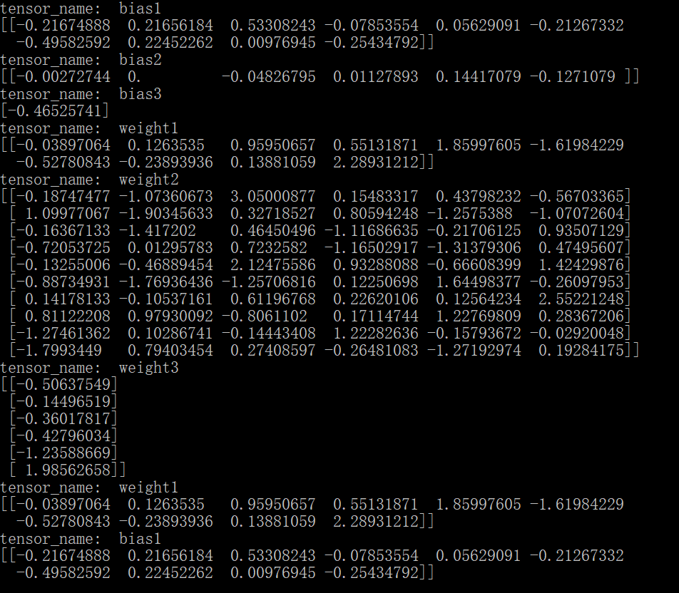
- #显示全部变量的名字和值
- chkp.print_tensors_in_checkpoint_file("model/mymodel.cpkt-5000", all_tensor_names='', tensor_name='', all_tensors=True)
- #显示指定名字变量的值
- chkp.print_tensors_in_checkpoint_file("model/mymodel.cpkt-5000", all_tensor_names='', tensor_name='weight1', all_tensors=False)
- chkp.print_tensors_in_checkpoint_file("model/mymodel.cpkt-5000", all_tensor_names='', tensor_name='bias1', all_tensors=False)
运行结果如下图:
相反如果对不同变量的操作用了同一个name,系统将会自动对同名称操作排序,例如:
- # -*- coding: utf-8 -*-
- import tensorflow as tf
- from tensorflow.python.tools import inspect_checkpoint as chkp
- #显示全部变量的名字和值
- chkp.print_tensors_in_checkpoint_file("model/mymodel.cpkt-50", all_tensor_names='', tensor_name='', all_tensors=True)
- #显示指定名字变量的值
- chkp.print_tensors_in_checkpoint_file("model/mymodel.cpkt-50", all_tensor_names='', tensor_name='weight', all_tensors=False)
- chkp.print_tensors_in_checkpoint_file("model/mymodel.cpkt-50", all_tensor_names='', tensor_name='bias', all_tensors=False)
结果为:
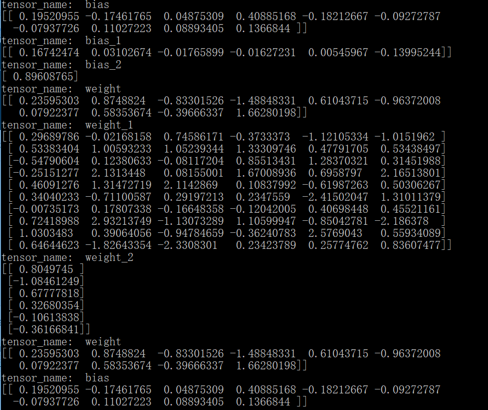
需要注意的是因为对所有同名的变量排序之后,真正的变量名已经变了,所以,当指定查看某一个变量的值时,其实输出的是第一个变量的值,因为它的名称还保留着不变。另外,也可以通过变量的name属性查看其操作名。
- 按名字保存变量
可以通过指定名称来保存变量;注意如果名字如果搞混了,名称所对应的值也就搞混了,比如:
- #只保存这两个变量,并且这两个被搞混了
- saver = tf.train.Saver({'weight': parameter['b2'], 'bias':parameter['W1']})
- # -*- coding: utf-8 -*-
- import tensorflow as tf
- from tensorflow.python.tools import inspect_checkpoint as chkp
- #显示全部变量的名字和值
- chkp.print_tensors_in_checkpoint_file("model/mymodel.cpkt-50", all_tensor_names='', tensor_name='', all_tensors=True)
- #显示指定名字变量的值
- chkp.print_tensors_in_checkpoint_file("model/mymodel.cpkt-50", all_tensor_names='', tensor_name='weight', all_tensors=False)
- chkp.print_tensors_in_checkpoint_file("model/mymodel.cpkt-50", all_tensor_names='', tensor_name='bias', all_tensors=False)
此时的结果是:
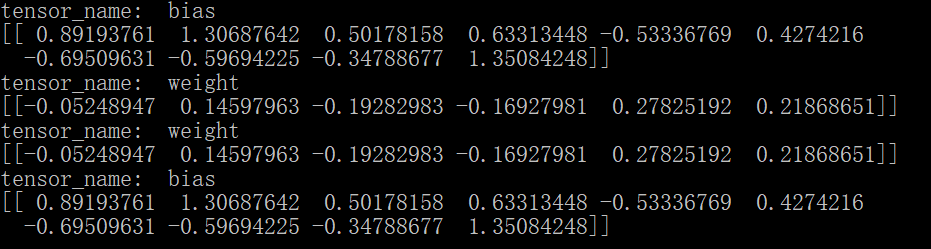
这样,模型按照我们的想法保存了参数,注意不能搞混变量和其对应的名字。
tensorflow神经网络拟合非线性函数与操作指南的更多相关文章
- 使用MindSpore的线性神经网络拟合非线性函数
技术背景 在前面的几篇博客中,我们分别介绍了MindSpore的CPU版本在Docker下的安装与配置方案.MindSpore的线性函数拟合以及MindSpore后来新推出的GPU版本的Docker编 ...
- 最小二乘法拟合非线性函数及其Matlab/Excel 实现(转)
1.最小二乘原理 Matlab直接实现最小二乘法的示例: close x = 1:1:100; a = -1.5; b = -10; y = a*log(x)+b; yrand = y + 0.5*r ...
- 最小二乘法拟合非线性函数及其Matlab/Excel 实现
1.最小二乘原理 Matlab直接实现最小二乘法的示例: close x = 1:1:100; a = -1.5; b = -10; y = a*log(x)+b; yrand = y + 0.5*r ...
- BP神经网络拟合给定函数
近期在准备美赛,因为比赛需要故重新安装了matlab,在里面想尝试一下神将网络工具箱.就找了一个看起来还挺赏心悦目的函数例子练练手: y=1+sin(1+pi*x/4) 针对这个函数,我们首先画出其在 ...
- MATLAB神经网络(2) BP神经网络的非线性系统建模——非线性函数拟合
2.1 案例背景 在工程应用中经常会遇到一些复杂的非线性系统,这些系统状态方程复杂,难以用数学方法准确建模.在这种情况下,可以建立BP神经网络表达这些非线性系统.该方法把未知系统看成是一个黑箱,首先用 ...
- MATLAB神经网络(3) 遗传算法优化BP神经网络——非线性函数拟合
3.1 案例背景 遗传算法(Genetic Algorithms)是一种模拟自然界遗传机制和生物进化论而形成的一种并行随机搜索最优化方法. 其基本要素包括:染色体编码方法.适应度函数.遗传操作和运行参 ...
- 『TensorFlow』第二弹_线性拟合&神经网络拟合_恰是故人归
Step1: 目标: 使用线性模拟器模拟指定的直线:y = 0.1*x + 0.3 代码: import tensorflow as tf import numpy as np import matp ...
- MATLAB神经网络(4) 神经网络遗传算法函数极值寻优——非线性函数极值寻优
4.1 案例背景 \[y = {x_1}^2 + {x_2}^2\] 4.2 模型建立 神经网络训练拟合根据寻优函数的特点构建合适的BP神经网络,用非线性函数的输入输出数据训练BP神经网络,训练后的B ...
- 非线性函数的最小二乘拟合及在Jupyter notebook中输入公式 [原创]
突然有个想法,能否通过学习一阶RC电路的阶跃响应得到RC电路的结构特征——时间常数τ(即R*C).回答无疑是肯定的,但问题是怎样通过最小二乘法.正规方程,以更多的采样点数来降低信号采集噪声对τ估计值的 ...
随机推荐
- selenium之安装和登陆操作举例
安装selenium: python -m pip install selenium-3.4.3-py2.py3-none-any.whl 下载对应浏览器版本的驱动,且在环境变量PATH中指定驱动程序 ...
- Highcharts之折线图
<!DOCTYPE html> <html> <head> <meta charset="UTF-8"> <title> ...
- python异常提示表
Python常见的异常提示及含义对照表如下: 异常名称 描述 BaseException 所有异常的基类 SystemExit 解释器请求退出 KeyboardInterrupt 用户中断执行(通常是 ...
- MT【70】图论的一些基本概念例题介绍
此讲是纯粹竞赛,联赛二试题难度.仅供学有余力的学生看看.
- 自学Linux Shell12.8-循环实例
点击返回 自学Linux命令行与Shell脚本之路 12.8-循环实例 待定. 3 fi bash shell的if语句会运行if后面的那个命令. 如果该命令的退出状态码是0 (该命令成功运行),位于 ...
- 自学Linux Shell15.1-处理信号
点击返回 自学Linux命令行与Shell脚本之路 15.1-处理信号 Linux使用信号与系统上运行的进程进行通信.可以使用这些信号控制Shell脚本的运行,只需要让shell脚本在接收到来自Lin ...
- 【AGC016E】Poor Turkeys
Description 有\(n\)(\(1 \le n \le 400\))只鸡,接下来按顺序进行\(m\)(\(1 \le m \le 10^5\))次操作.每次操作涉及两只鸡,如果都存在则随意拿 ...
- K8s核心概念详解
kubernetes(通常简称为K8S),是一个用于管理在容器中运行的应用的容器编排工具. Kubernetes不仅有你所需要的用来支持复杂容器应用的所有东西,它还是市面上最方便开发和运维的框架. K ...
- qsort代码(pascal/c/c++)与思想及扩展(随机化,TopK)
1.快速排序思想:从一堆数A中找到一个数x,然后把这堆数x分成两堆B,C,B堆的数小于(或小于等于)该数,放在左边,C堆的数大于(或大于等于)该数,放在右边,有可能把该数x单独分开,放在中间.然后对小 ...
- ps 中取消网格线的吸附功能,其实是对齐功能
ps 中取消网格线的吸附功能,其实是对齐功能